SAGA: A Fast Incremental Gradient Method With Support for Non-Strongly Convex Composite Objectives

SAGA: 一种支持非强凸复合目标的快速增量梯度方法

Aaron Defazio Ambiata ∗ Australian National University, Canberra

Aaron Defazio Ambiata ∗ 澳大利亚国立大学，堪培拉

Francis Bach INRIA - Sierra Project-Team Ecole Normale Superieure, Paris, France

Francis Bach INRIA - Sierra 项目团队 巴黎高等师范学院，法国

Simon Lacoste-Julien INRIA - Sierra Project-Team Ecole Normale Superieure, Paris, France

Simon Lacoste-Julien INRIA - Sierra 项目团队 巴黎高等师范学院，法国

Abstract

摘要

In this work we introduce a new optimisation method called SAGA in the spirit of SAG, SDCA, MISO and SVRG, a set of recently proposed incremental gradient algorithms with fast linear convergence rates. SAGA improves on the theory behind SAG and SVRG, with better theoretical convergence rates, and has support for composite objectives where a proximal operator is used on the regular is er. Unlike SDCA, SAGA supports non-strongly convex problems directly, and is adaptive to any inherent strong convexity of the problem. We give experimental results showing the effectiveness of our method.

在本工作中，我们引入了一种名为 SAGA 的新优化方法，其灵感来源于 SAG、SDCA、MISO 和 SVRG，这些是最近提出的一组具有快速线性收敛速度的增量梯度算法。SAGA 在 SAG 和 SVRG 的理论基础上进行了改进，具有更好的理论收敛速度，并且支持在正则化项上使用近端算子的复合目标。与 SDCA 不同，SAGA 直接支持非强凸问题，并且能够自适应问题的任何内在强凸性。我们提供了实验结果，展示了该方法的有效性。

1 Introduction

1 引言

Remarkably, recent advances [1, 2] have shown that it is possible to minimise strongly convex finite sums provably faster in expectation than is possible without the finite sum structure. This is significant for machine learning problems as a finite sum structure is common in the empirical risk minim is ation setting. The requirement of strong convexity is likewise satisfied in machine learning problems in the typical case where a quadratic regular is er is used.

值得注意的是，最近的进展 [1, 2] 表明，在期望值上，可以比没有有限和结构的情况下更快地最小化强凸有限和。这对于机器学习问题具有重要意义，因为在经验风险最小化设置中，有限和结构是常见的。在机器学习问题中，强凸性要求通常在使用二次正则化器的情况下得到满足。

In particular, we are interested in minimising functions of the form

我们特别关注最小化以下形式的函数

where $\boldsymbol{x}\in\mathbb{R}^{d}$ , each $f_{i}$ is convex and has Lipschitz continuous derivatives with constant $L$ . We will also consider the case where each $f_{i}$ is strongly convex with constant $\mu$ , and the “composite” (or proximal) case where an additional regular is ation function is added:

其中 $\boldsymbol{x}\in\mathbb{R}^{d}$，每个 $f_{i}$ 是凸函数，并且具有 Lipschitz 连续导数，常数为 $L$。我们还将考虑每个 $f_{i}$ 是强凸函数，常数为 $\mu$ 的情况，以及“复合”（或近端）情况，其中添加了额外的正则化函数：

where $h\colon\ensuremath{\mathbb{R}}^{d}\to\ensuremath{\mathbb{R}}^{d}$ is convex but potentially non-differentiable, and where the proximal operation of $h$ is easy to compute — few incremental gradient methods are applicable in this setting [3][4].

其中 $h\colon\ensuremath{\mathbb{R}}^{d}\to\ensuremath{\mathbb{R}}^{d}$ 是凸函数但可能不可微，且 $h$ 的近端操作易于计算——在这种设置下，很少有增量梯度方法适用 [3][4]。

Our contributions are as follows. In Section 2 we describe the SAGA algorithm, a novel incremental gradient method. In Section 5 we prove theoretical convergence rates for SAGA in the strongly convex case better than those for SAG [1] and SVRG [5], and a factor of 2 from the SDCA [2] convergence rates. These rates also hold in the composite setting. Additionally, we show that like SAG but unlike SDCA, our method is applicable to non-strongly convex problems without modification. We establish theoretical convergence rates for this case also. In Section 3 we discuss the relation between each of the fast incremental gradient methods, showing that each stems from a very small modification of another.

我们的贡献如下。在第2节中，我们描述了SAGA算法，这是一种新颖的增量梯度方法。在第5节中，我们证明了SAGA在强凸情况下的理论收敛速度优于SAG [1] 和 SVRG [5]，并且与SDCA [2] 的收敛速度相差2倍。这些速度在复合设置中也成立。此外，我们展示了与SAG类似但与SDCA不同的是，我们的方法无需修改即可适用于非强凸问题。我们也为这种情况建立了理论收敛速度。在第3节中，我们讨论了每种快速增量梯度方法之间的关系，表明每种方法都是对另一种方法的微小修改。

2 SAGA Algorithm

2 SAGA 算法

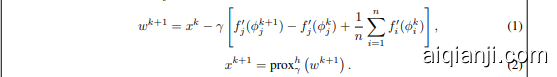
We start with some known initial vector $x^{0}\in\mathbb{R}^{d}$ and known derivatives $f_{i}^{\prime}(\phi_{i}^{0})\in\mathbb{R}^{d}$ with $\phi_{i}^{0}=x^{0}$ for each $i$ . These derivatives are stored in a table data-structure of length $n$ , or alternatively a $n\times d$ matrix. For many problems of interest, such as binary classification and least-squares, only a single floating point value instead of a full gradient vector needs to be stored (see Section 4). SAGA is inspired both from SAG [1] and SVRG [5] (as we will discuss in Section 3). SAGA uses a step size of $\gamma$ and makes the following updates, starting with $k=0$ :

我们从已知的初始向量 $x^{0}\in\mathbb{R}^{d}$ 和已知的导数 $f_{i}^{\prime}(\phi_{i}^{0})\in\mathbb{R}^{d}$ 开始，其中 $\phi_{i}^{0}=x^{0}$ 对于每个 $i$。这些导数存储在一个长度为 $n$ 的表数据结构中，或者存储在一个 $n\times d$ 的矩阵中。对于许多感兴趣的问题，如二分类和最小二乘法，只需要存储一个浮点值，而不是完整的梯度向量（见第4节）。SAGA 的灵感来自 SAG [1] 和 SVRG [5]（我们将在第3节讨论）。SAGA 使用步长 $\gamma$，并从 $k=0$ 开始进行以下更新：

SAGA Algorithm: Given the value of $x^{k}$ and of each $f_{i}^{\prime}(\phi_{i}^{k})$ at the end of iteration $k$ , the updates for iteration $k+1$ is as follows:

SAGA 算法：给定迭代 $k$ 结束时的 $x^{k}$ 和每个 $f_{i}^{\prime}(\phi_{i}^{k})$ 的值，迭代 $k+1$ 的更新如下：

3. Update $x$ using $f_{j}^{\prime}(\phi_{j}^{k+1})$ , $f_{j}^{\prime}(\phi_{j}^{k})$ and the table average:
4. 使用 $f_{j}^{\prime}(\phi_{j}^{k+1})$ 、 $f_{j}^{\prime}(\phi_{j}^{k})$ 和表格平均值更新 $x$：

The proximal operator we use above is defined as

我们上面使用的近端算子定义为

In the strongly convex case, when a step size of $\gamma=1/(2(\mu n+L))$ is chosen, we have the following convergence rate in the composite and hence also the non-composite case:

在强凸情况下，当选择步长 $\gamma=1/(2(\mu n+L))$ 时，我们在复合情况（因此也包括非复合情况）下有以下收敛率：

We prove this result in Section 5. The requirement of strong convexity can be relaxed from needing to hold for each $f_{i}$ to just holding on average, but at the expense of a worse geometric rate $(1-$ 6(µnµ+L) ), requiring a step size of γ = 1/(3(µn + L)).

我们在第5节中证明了这一结果。强凸性的要求可以从每个$f_{i}$都需要满足，放宽为仅在平均意义上满足，但代价是几何速率变差$(1-$6(µnµ+L) )，需要步长γ = 1/(3(µn + L))。

In the non-strongly convex case, we have established the convergence rate in terms of the average iterate, excluding step 0: $\begin{array}{r}{\bar{x}^{k}=\frac{1}{k}\sum_{t=1}^{k}x^{t}}\end{array}$ . Using a step size of $\gamma=1/(3L)$ we have

在非强凸情况下，我们建立了关于平均迭代的收敛速度（不包括第0步）：$\begin{array}{r}{\bar{x}^{k}=\frac{1}{k}\sum_{t=1}^{k}x^{t}}\end{array}$。使用步长 $\gamma=1/(3L)$，我们有

This result is proved in the supplementary material. Importantly, when this step size $\gamma=1/(3L)$ is used, our algorithm automatically adapts to the level of strong convexity $\mu>0$ naturally present, giving a convergence rate of (see the comment at the end of the proof of Theorem 1):

该结果在补充材料中得到了证明。重要的是，当使用步长 $\gamma=1/(3L)$ 时，我们的算法会自动适应自然存在的强凸性水平 $\mu>0$，从而给出以下收敛速度（参见定理 1 证明末尾的评论）：

Although any incremental gradient method can be applied to non-strongly convex problems via the addition of a small quadratic regular is ation, the amount of regular is ation is an additional tunable parameter which our method avoids.

虽然任何增量梯度方法都可以通过添加一个小的二次正则化项应用于非强凸问题，但正则化的量是一个额外的可调参数，而我们的方法避免了这一点。

3 Related Work

3 相关工作

We explore the relationship between SAGA and the other fast incremental gradient methods in this section. By using SAGA as a midpoint, we are able to provide a more unified view than is available in the existing literature. A brief summary of the properties of each method considered in this section is given in Figure 1. The method from [3], which handles the non-composite setting, is not listed as its rate is of the slow type and can be up to $n$ times smaller than the one for SAGA or SVRG [5].

在本节中，我们探讨了 SAGA 与其他快速增量梯度方法之间的关系。通过将 SAGA 作为中间点，我们能够提供一个比现有文献更为统一的视角。图 1 给出了本节中考虑的每种方法的简要特性总结。[3] 中的方法处理的是非复合设置，未列出，因为其收敛速度较慢，可能比 SAGA 或 SVRG [5] 的收敛速度慢至 $n$ 倍。

	SAGA	SAG	SDCA	SVRG	FINITO
强凸 (SC)
凸, 非强凸 (Non-SC)*			×	？	？
近端正则 (Prox Reg.)		？	/[6]
非光滑 (Non-smooth)		X			×
低存储成本 (LowStorage eCost)	×	×		√	×
简单证明 (Simple(-ish) Proof)	√		√	√
自适应强凸 (AdaptivetoSC)			x	？	？

SAGA: midpoint between SAG and SVRG/S2GD

SAGA：SAG 与 SVRG/S2GD 之间的中点

In [5], the authors make the observation that the variance of the standard stochastic gradient (SGD) update direction can only go to zero if decreasing step sizes are used, thus preventing a linear convergence rate unlike for batch gradient descent. They thus propose to use a variance reduction approach (see [7] and references therein for example) on the SGD update in order to be able to use constant step sizes and get a linear convergence rate. We present the updates of their method called SVRG (Stochastic Variance Reduced Gradient) in (6) below, comparing it with the non-composite form of SAGA rewritten in (5). They also mention that SAG (Stochastic Average Gradient) [1] can be interpreted as reducing the variance, though they do not provide the specifics. Here, we make this connection clearer and relate it to SAGA.

在 [5] 中，作者观察到，标准随机梯度下降 (SGD) 更新方向的方差只有在使用递减步长时才能趋近于零，因此无法像批量梯度下降那样实现线性收敛速度。因此，他们提出在 SGD 更新中使用方差缩减方法（例如参见 [7] 及其参考文献），以便能够使用恒定步长并获得线性收敛速度。我们在下面的 (6) 中展示了他们提出的 SVRG (Stochastic Variance Reduced Gradient) 方法的更新，并将其与重写为 (5) 的非复合形式的 SAGA 进行比较。他们还提到，SAG (Stochastic Average Gradient) [1] 可以被解释为减少方差的方法，尽管他们没有提供具体细节。在这里，我们更清晰地阐述了这种联系，并将其与 SAGA 相关联。

We first review a slightly more generalized version of the variance reduction approach (we allow the updates to be biased). Suppose that we want to use Monte Carlo samples to estimate $\mathbb{E}X$ and that we can compute efficiently $\mathbb{E}Y$ for another random variable $Y$ that is highly correlated with $X$ . One variance reduction approach is to use the following estimator $\theta_{\alpha}$ as an approximation to $\mathbb{E}X\colon\theta_{\alpha}:=$ $\alpha(X-Y)+\mathbb{E}Y.$ , for a step size $\alpha\in[0,1]$ . We have that $\mathbb{E}\theta_{\alpha}$ is a convex combination of $\mathbb{E}X$ and $\mathbb{E}Y$ : $\mathbb{E}\theta_{\alpha}=\alpha\mathbb{E}X+(1-\alpha)\mathbb{E}Y$ . The standard variance reduction approach uses $\alpha=1$ and the estimate is unbiased $\mathbb{E}\theta_{1}=\mathbb{E}X$ . The variance of $\theta_{\alpha}$ is: $\operatorname{Var}(\theta_{\alpha})=\alpha^{2}[\operatorname{Var}(X)+\operatorname{Var}(Y)-2\operatorname{Cov}(X,Y)].$ , and so if $\operatorname{Cov}(X,Y)$ is big enough, the variance of $\theta_{\alpha}$ is reduced compared to $X$ , giving the method its name. By varying $\alpha$ from 0 to 1, we increase the variance of $\theta_{\alpha}$ towards its maximum value (which usually is still smaller than the one for $X$ ) while decreasing its bias towards zero.

我们首先回顾一个稍微更广义的方差减少方法版本（我们允许更新是有偏的）。假设我们想使用蒙特卡洛样本来估计 $\mathbb{E}X$，并且我们可以高效地计算另一个与 $X$ 高度相关的随机变量 $Y$ 的 $\mathbb{E}Y$。一种方差减少方法是使用以下估计器 $\theta_{\alpha}$ 作为 $\mathbb{E}X$ 的近似值：$\theta_{\alpha}:=$ $\alpha(X-Y)+\mathbb{E}Y.$，其中步长 $\alpha\in[0,1]$。我们有 $\mathbb{E}\theta_{\alpha}$ 是 $\mathbb{E}X$ 和 $\mathbb{E}Y$ 的凸组合：$\mathbb{E}\theta_{\alpha}=\alpha\mathbb{E}X+(1-\alpha)\mathbb{E}Y$。标准的方差减少方法使用 $\alpha=1$，估计是无偏的 $\mathbb{E}\theta_{1}=\mathbb{E}X$。$\theta_{\alpha}$ 的方差为：$\operatorname{Var}(\theta_{\alpha})=\alpha^{2}[\operatorname{Var}(X)+\operatorname{Var}(Y)-2\operatorname{Cov}(X,Y)].$，因此如果 $\operatorname{Cov}(X,Y)$ 足够大，$\theta_{\alpha}$ 的方差相比 $X$ 会减小，这也是该方法名称的由来。通过将 $\alpha$ 从 0 变化到 1，我们增加 $\theta_{\alpha}$ 的方差趋向其最大值（通常仍小于 $X$ 的方差），同时减少其偏差趋向于零。

Both SAGA and SAG can be derived from such a variance reduction viewpoint: here $X$ is the SGD direction sample $f_{j}^{\prime}(x^{k})$ , whereas $Y$ is a past stored gradient $f_{j}^{\prime}(\phi_{j}^{k})$ . SAG is obtained by using $\alpha=1/n$ (update rewritten in our notation in (4)), whereas SAGA is the unbiased version with $\alpha=1$ (see (5) below). For the same $\phi$ ’s, the variance of the SAG update is $1/n^{2}$ times the one of SAGA, but at the expense of having a non-zero bias. This non-zero bias might explain the complexity of the convergence proof of SAG and why the theory has not yet been extended to proximal operators. By using an unbiased update in SAGA, we are able to obtain a simple and tight theory, with better constants than SAG, as well as theoretical rates for the use of proximal operators.

SAGA 和 SAG 都可以从方差减少的角度推导出来：这里 $X$ 是 SGD 方向的样本 $f_{j}^{\prime}(x^{k})$，而 $Y$ 是过去存储的梯度 $f_{j}^{\prime}(\phi_{j}^{k})$。SAG 通过使用 $\alpha=1/n$ 获得（在我们的符号中重写为 (4)），而 SAGA 是无偏版本，使用 $\alpha=1$（见下面的 (5)）。对于相同的 $\phi$，SAG 更新的方差是 SAGA 的 $1/n^{2}$ 倍，但代价是存在非零偏差。这种非零偏差可能解释了 SAG 收敛证明的复杂性，以及为什么该理论尚未扩展到近端算子。通过在 SAGA 中使用无偏更新，我们能够获得一个简单且紧密的理论，其常数优于 SAG，并且还提供了使用近端算子的理论速率。

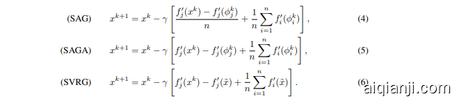
The SVRG update (6) is obtained by using $Y=f_{j}^{\prime}(\tilde{x})$ with $\alpha=1$ (and is thus unbiased – we note that SAG is the only method that we present in the related work that has a biased update direction). The vector $\tilde{x}$ is not updated every step, but rather the loop over $k$ appears inside an outer loop, where $\tilde{x}$ is updated at the start of each outer iteration. Essentially SAGA is at the midpoint between SVRG and SAG; it updates the $\phi_{j}$ value each time index $j$ is picked, whereas SVRG updates all of $\phi$ ’s as a batch. The S2GD method [8] has the same update as SVRG, just differing in how the number of inner loop iterations is chosen. We use SVRG henceforth to refer to both methods.

SVRG 更新 (6) 是通过使用 $Y=f_{j}^{\prime}(\tilde{x})$ 且 $\alpha=1$ 得到的（因此是无偏的——我们注意到 SAG 是我们在相关工作中展示的唯一一种具有有偏更新方向的方法）。向量 $\tilde{x}$ 并不是每一步都更新，而是在一个外部循环中更新，其中 $\tilde{x}$ 在每次外部迭代开始时更新。本质上，SAGA 位于 SVRG 和 SAG 之间的中点；它每次选择索引 $j$ 时都会更新 $\phi_{j}$ 值，而 SVRG 则批量更新所有 $\phi$ 值。S2GD 方法 [8] 的更新与 SVRG 相同，只是内部循环迭代次数的选择方式不同。我们此后使用 SVRG 来指代这两种方法。

SVRG makes a trade-off between time and space. For the equivalent practical convergence rate it makes $2\mathbf{x}{\mathbf{-}}3\mathbf{x}$ more gradient evaluations, but in doing so it does not need to store a table of gradients, but a single average gradient. The usage of SAG vs. SVRG is problem dependent. For example for linear predictors where gradients can be stored as a reduced vector of dimension $p-1$ for $p$ classes, SAGA is preferred over SVRG both theoretically and in practice. For neural networks, where no theory is available for either method, the storage of gradients is generally more expensive than the additional back propagation s, but this is computer architecture dependent.

SVRG 在时间和空间之间做出了权衡。为了达到相同的实际收敛速度，它需要进行 $2\mathbf{x}{\mathbf{-}}3\mathbf{x}$ 次梯度评估，但这样做不需要存储梯度表，而是存储一个平均梯度。SAG 与 SVRG 的使用取决于具体问题。例如，对于线性预测器，梯度可以存储为维度为 $p-1$ 的缩减向量（对于 $p$ 个类别），SAGA 在理论上和实践中都优于 SVRG。对于神经网络，由于这两种方法都没有理论支持，存储梯度的成本通常比额外的反向传播更高，但这取决于计算机架构。

SVRG also has an additional parameter besides step size that needs to be set, namely the number of iterations per inner loop $(m)$ . This parameter can be set via the theory, or conservatively as $m=n$ , however doing so does not give anywhere near the best practical performance. Having to tune one parameter instead of two is a practical advantage for SAGA.

SVRG 除了步长外还有一个需要设置的额外参数，即每个内循环的迭代次数 $(m)$。这个参数可以通过理论设置，或者保守地设置为 $m=n$，但这样做并不能达到最佳的实际性能。对于 SAGA 来说，只需调整一个参数而不是两个，这是一个实际的优势。

Finito/MISOµ

Finito/MISOµ

To make the relationship with other prior methods more apparent, we can rewrite the SAGA algorithm (in the non-composite case) in term of an additional intermediate quantity $u^{k}$ , with $\begin{array}{r}{u^{\tilde{0}}:=x^{0}+\gamma\sum_{i=1}^{n}f_{i}^{\prime}(x^{0})}\end{array}$ , in addition to the usual $x^{k}$ iterate as described previously:

为了使与其他先前方法的关系更加明显，我们可以在非复合情况下重写SAGA算法，引入一个额外的中间量 $u^{k}$ ，除了之前描述的常规 $x^{k}$ 迭代外，还有 $\begin{array}{r}{u^{\tilde{0}}:=x^{0}+\gamma\sum_{i=1}^{n}f_{i}^{\prime}(x^{0})}\end{array}$ 。

SAGA: Equivalent reformulation for non-composite case: Given the value of $u^{k}$ and of each $f_{i}^{\prime}(\phi_{i}^{k})$ at the end of iteration $k$ , the updates for iteration $k+1$ , is as follows:

SAGA：非复合情况下的等价重构：给定迭代 $k$ 结束时 $u^{k}$ 和每个 $f_{i}^{\prime}(\phi_{i}^{k})$ 的值，迭代 $k+1$ 的更新如下：

1. Calculate $x^{k}$ :
2. 计算 $x^{k}$ :

2. Update $u$ with $\begin{array}{r}{u^{k+1}=u^{k}+\frac{1}{n}(x^{k}-u^{k})}\end{array}$ .
3. 更新 $u$ 为 $\begin{array}{r}{u^{k+1}=u^{k}+\frac{1}{n}(x^{k}-u^{k})}\end{array}$。
4. Pick a $j$ uniformly at random.
5. 随机均匀选择一个 $j$。
6. Take $\phi_{j}^{k+1}=x^{k}$ , and store $f_{j}^{\prime}(\phi_{j}^{k+1})$ in the table replacing $f_{j}^{\prime}(\phi_{j}^{k})$ . All other entries in the table remain unchanged. The quantity $\phi_{j}^{k+1}$ is not explicitly stored.
7. 取 $\phi_{j}^{k+1}=x^{k}$，并将 $f_{j}^{\prime}(\phi_{j}^{k+1})$ 存储在表中，替换 $f_{j}^{\prime}(\phi_{j}^{k})$。表中的其他条目保持不变。量 $\phi_{j}^{k+1}$ 不显式存储。

Eliminating $u^{k}$ recovers the update (5) for $x^{k}$ . We now describe how the Finito [9] and ${\bf M}{\bf S}{\bf O}\mu$ [10] methods are closely related to SAGA. Both Finito and ${\bf M}{\bf S}{\bf O}\mu$ use updates of the following form, for a step length $\gamma$ :

消除 $u^{k}$ 后，我们恢复了 $x^{k}$ 的更新 (5)。现在我们将描述 Finito [9] 和 ${\bf M}{\bf S}{\bf O}\mu$ [10] 方法与 SAGA 的密切关系。Finito 和 ${\bf M}{\bf S}{\bf O}\mu$ 都使用以下形式的更新，步长为 $\gamma$：

The step size used is of the order of $1/\mu n$ . To simplify the discussion of this algorithm we will introduce the notation $\begin{array}{r}{\bar{\phi}=\frac{1}{n}\sum_{i}\phi_{i}^{k}}\end{array}$ .

使用的步长约为 $1/\mu n$。为了简化对该算法的讨论，我们将引入符号 $\begin{array}{r}{\bar{\phi}=\frac{1}{n}\sum_{i}\phi_{i}^{k}}\end{array}$。

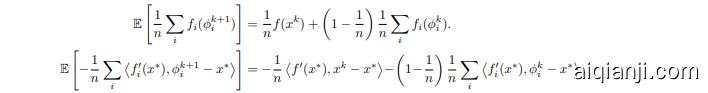
SAGA can be interpreted as Finito, but with the quantity $\bar{\phi}$ replaced with $u$ , which is updated in the same way as $\bar{\phi}$ , but in expectation. To see this, consider how $\phi$ changes in expectation:

SAGA 可以解释为 Finito，但将量 $\bar{\phi}$ 替换为 $u$，并以与 $\bar{\phi}$ 相同的方式更新，但在期望中。为了理解这一点，考虑 $\phi$ 在期望中如何变化：

The update is identical in expectation to the update for $u$ , $\begin{array}{r}{u^{k+1}=u^{k}+\frac{1}{n}(x^{k}-u^{k})}\end{array}$ . There are three advantages of SAGA over Finito $/\mathbf{M}\mathbf{S}\mathbf{O}\mu$ . SAGA does not require strong convexity to work, it has support for proximal operators, and it does not require storing the $\phi_{i}$ values. MISO has proven support for proximal operators only in the case where im practically small step sizes are used [10]. The big advantage of Finito $/{\bf M}\mathrm{SO}\mu$ is that when using a per-pass re-permuted access ordering, empirical speed-ups of up-to a factor of $2\mathbf{x}$ has been observed. This access order can also be used with the other methods discussed, but with smaller empirical speed-ups. Finito $/\mathbf{M}\mathbf{S}\mathbf{O}\mu$ is particularly useful when $f_{i}$ is computationally expensive to compute compared to the extra storage costs required over the other methods.

更新在期望上与 $u$ 的更新相同，即 $\begin{array}{r}{u^{k+1}=u^{k}+\frac{1}{n}(x^{k}-u^{k})}\end{array}$。SAGA 相对于 Finito $/\mathbf{M}\mathbf{S}\mathbf{O}\mu$ 有三个优势。SAGA 不需要强凸性即可工作，它支持近端算子，并且不需要存储 $\phi_{i}$ 值。MISO 仅在使用了非常小的步长的情况下证明了其对近端算子的支持 [10]。Finito $/{\bf M}\mathrm{SO}\mu$ 的最大优势在于，当使用每遍重新排列的访问顺序时，经验上观察到速度提升可达 $2\mathbf{x}$ 倍。这种访问顺序也可以用于其他讨论的方法，但经验上的速度提升较小。当 $f_{i}$ 的计算成本相对于其他方法所需的额外存储成本较高时，Finito $/\mathbf{M}\mathbf{S}\mathbf{O}\mu$ 特别有用。

SDCA

SDCA

The Stochastic Dual Coordinate Descent (SDCA) [2] method on the surface appears quite different from the other methods considered. It works with the convex conjugates of the $f_{i}$ functions. However, in this section we show a novel transformation of SDCA into an equivalent method that only works with primal quantities, and is closely related to the ${\bf M}{\bf S}{\bf O}\mu$ method.

随机对偶坐标下降法 (Stochastic Dual Coordinate Descent, SDCA) [2] 在表面上看起来与其他方法有很大不同。它通过 $f_{i}$ 函数的凸共轭来工作。然而，在本节中，我们展示了将 SDCA 转换为一种仅使用原始量的等效方法的新颖变换，并且该方法与 ${\bf M}{\bf S}{\bf O}\mu$ 方法密切相关。

Consider the following algorithm:

考虑以下算法：

SDCA algorithm in the primal

SDCA 算法在原始问题中的应用

Step $k+1$ :

步骤 $k+1$：

At completion, return $\begin{array}{r}{x^{k}=-\gamma\sum_{i}^{n}f_{i}^{\prime}(\phi_{i}^{k})}\end{array}$ .

完成后，返回 $\begin{array}{r}{x^{k}=-\gamma\sum_{i}^{n}f_{i}^{\prime}(\phi_{i}^{k})}\end{array}$。

We claim that this algorithm is equivalent to the version of SDCA where exact block-coordinate maxim is ation is used on the dual.1 Firstly, note that while SDCA was originally described for onedimensional outputs (binary classification or regression), it has been expanded to cover the multiclass predictor case [11] (called Prox-SDCA there). In this case, the primal objective has a separate strongly convex regular is er, and the functions $f_{i}$ are restricted to the form $f_{i}(x)\dot{}=\psi_{i}(X_{i}^{T}x)$ , where $X_{i}$ is a $d\times p$ feature matrix, and $\psi_{i}$ is the loss function that takes a $p$ dimensional input, for $p$ classes. To stay in the same general setting as the other incremental gradient methods, we work directly with the $f_{i}(x)$ functions rather than the more structured $\psi_{i}(X_{i}^{T}\bar{x})$ . The dual objective to maximise then becomes

我们声称该算法等同于在双问题上使用精确块坐标最大化的SDCA版本。首先，注意到虽然SDCA最初是为单维输出（二分类或回归）描述的，但它已被扩展以涵盖多类预测器的情况 [11]（在那里称为Prox-SDCA）。在这种情况下，原始目标函数具有单独的强凸正则项，函数 $f_{i}$ 被限制为 $f_{i}(x)\dot{}=\psi_{i}(X_{i}^{T}x)$ 的形式，其中 $X_{i}$ 是一个 $d\times p$ 的特征矩阵，$\psi_{i}$ 是接受 $p$ 维输入的损失函数，用于 $p$ 个类别。为了与其他增量梯度方法保持相同的通用设置，我们直接使用 $f_{i}(x)$ 函数，而不是更具结构性的 $\psi_{i}(X_{i}^{T}\bar{x})$。要最大化的双目标函数则变为

$$
D(\alpha)=\left[-\frac{\mu}{2}\left|\frac{1}{\mu n}\sum_{i=1}^{n}\alpha_{i}\right|^{2}-\frac{1}{n}\sum_{i=1}^{n}f_{i}^{*}(-\alpha_{i})\right],
$$

$$
D(\alpha)=\left[-\frac{\mu}{2}\left|\frac{1}{\mu n}\sum_{i=1}^{n}\alpha_{i}\right|^{2}-\frac{1}{n}\sum_{i=1}^{n}f_{i}^{*}(-\alpha_{i})\right],
$$

where $\alpha_{i}$ ’s are $d$ -dimensional dual variables. General ising the exact block-coordinate maxim is ation update that SDCA performs to this form, we get the dual update for block $j$ (with $x^{k}$ the current primal iterate):

其中 $\alpha_{i}$ 是 $d$ 维对偶变量。将 SDCA 执行的精确块坐标最大化更新推广到这种形式，我们得到块 $j$ 的对偶更新（其中 $x^{k}$ 是当前的主迭代）：

In the special case where $f_{i}(x)=\psi_{i}(X_{i}^{T}x)$ , we can see that (9) gives exactly the same update as Option I of Prox-SDCA in [11, Figure 1], which operates instead on the equivalent $p$ -dimensional dual variables $\tilde{\alpha}{i}$ with the relationship that $\alpha{i}=X_{i}\bar{\alpha}{i}$ .2 As noted by Shalev-Shwartz & Zhang [11], the update (9) is actually an instance of the proximal operator of the convex conjugate of $f{j}$ . Our primal formulation exploits this fact by using a relation between the proximal operator of a function and its convex conjugate known as the Moreau decomposition:

在特殊情况下，当 $f_{i}(x)=\psi_{i}(X_{i}^{T}x)$ 时，我们可以看到 (9) 给出的更新与 [11, 图 1] 中 Prox-SDCA 的选项 I 完全相同，后者在等价的 $p$ 维对偶变量 $\tilde{\alpha}{i}$ 上操作，且满足 $\alpha{i}=X_{i}\bar{\alpha}{i}$ 的关系。正如 Shalev-Shwartz & Zhang [11] 所指出的，更新 (9) 实际上是 $f{j}$ 的凸共轭的近端算子的一个实例。我们的原始公式通过利用函数与其凸共轭之间的 Moreau 分解关系来利用这一事实：

This decomposition allows us to compute the proximal operator of the conjugate via the primal proximal operator. As this is the only use in the basic SDCA method of the conjugate function, applying this decomposition allows us to completely eliminate the “dual” aspect of the algorithm, yielding the above primal form of SDCA. The dual variables are related to the primal representatives $\phi_{i}$ ’s through $\bar{\alpha_{i}}=-f_{i}^{\prime}(\phi_{i})$ . The KKT conditions ensure that if the $\alpha_{i}$ values are dual optimal then $\textstyle x^{k}=\gamma\sum_{i}\alpha_{i}$ as defined above is primal optimal. The same trick is commonly used to interpret Dijkst ra’s set intersection as a primal algorithm instead of a dual block coordinate descent algorithm [12].

这种分解使我们能够通过原始近端算子计算共轭的近端算子。由于这是基本SDCA方法中唯一使用共轭函数的地方，应用这种分解使我们能够完全消除算法的“对偶”方面，从而得到上述的原始形式SDCA。对偶变量通过 $\bar{\alpha_{i}}=-f_{i}^{\prime}(\phi_{i})$ 与原始代表 $\phi_{i}$ 相关联。KKT条件确保如果 $\alpha_{i}$ 值是对偶最优的，则如上定义的 $\textstyle x^{k}=\gamma\sum_{i}\alpha_{i}$ 是原始最优的。同样的技巧通常用于将Dijkstra的集合交集解释为原始算法，而不是对偶块坐标下降算法 [12]。

The primal form of SDCA differs from the other incremental gradient methods described in this section in that it assumes strong convexity is induced by a separate strongly convex regular is er, rather than each $f_{i}$ being strongly convex. In fact, SDCA can be modified to work without a separate regular is er, giving a method that is at the midpoint between Finito and SDCA. We detail such a method in the supplementary material.

SDCA的原始形式与本节中描述的其他增量梯度方法不同，它假设强凸性是由一个单独的强凸正则化器引入的，而不是每个 $f_{i}$ 都是强凸的。事实上，SDCA可以修改为在没有单独正则化器的情况下工作，从而得到一种介于Finito和SDCA之间的方法。我们在补充材料中详细描述了这种方法。

SDCA variants

SDCA 变体

The SDCA theory has been expanded to cover a number of other methods of performing the coordinate step [11]. These variants replace the proximal operation in our primal interpretation in the previous section with an update where $\phi_{j}^{k+1}$ is chosen so that: $f_{j}^{\prime}(\phi_{j}^{k+1})\stackrel{\leftarrow}{=}(1-\beta){f_{j}^{\prime}}(\phi_{j}^{k})+\beta f_{j}^{\prime}(x^{k})$ , where $\begin{array}{r}{x^{k}=-\frac{1}{\mu n}\sum_{i}f_{i}^{\prime}(\phi_{i}^{k})}\end{array}$ . The variants differ in how $\beta\in[0,1]$ is chosen. Note that $\phi_{j}^{k+1}$ does not actually have to be explicitly known, just the gradient $f_{j}^{\prime}(\phi_{j}^{k+1})$ , which is the result of the above interpolation. Variant 5 by Shalev-Shwartz & Zhang [11] does not require operations on the conjugate function, it simply uses $\textstyle\beta={\frac{\mu n}{L+\mu n}}$ . The most practical variant performs a line search involving the convex conjugate to determine $\beta$ . As far as we are aware, there is no simple primal equivalent of this line search. So in cases where we can not compute the proximal operator from the standard SDCA variant, we can either introduce a tuneable parameter into the algorithm $(\beta)$ , or use a dual line search, which requires an efficient way to evaluate the convex conjugates of each $f_{i}$ .

SDCA 理论已经扩展到涵盖执行坐标步骤的多种其他方法 [11]。这些变体将上一节中我们对原始解释的近端操作替换为更新，其中选择 $\phi_{j}^{k+1}$ 使得：$f_{j}^{\prime}(\phi_{j}^{k+1})\stackrel{\leftarrow}{=}(1-\beta){f_{j}^{\prime}}(\phi_{j}^{k})+\beta f_{j}^{\prime}(x^{k})$，其中 $\begin{array}{r}{x^{k}=-\frac{1}{\mu n}\sum_{i}f_{i}^{\prime}(\phi_{i}^{k})}\end{array}$。这些变体的区别在于如何选择 $\beta\in[0,1]$。需要注意的是，$\phi_{j}^{k+1}$ 实际上不需要显式已知，只需要梯度 $f_{j}^{\prime}(\phi_{j}^{k+1})$，这是上述插值的结果。Shalev-Shwartz & Zhang [11] 的变体 5 不需要对共轭函数进行操作，它简单地使用 $\textstyle\beta={\frac{\mu n}{L+\mu n}}$。最实用的变体通过涉及凸共轭的线搜索来确定 $\beta$。据我们所知，这种线搜索没有简单的原始等价形式。因此，在我们无法从标准 SDCA 变体计算近端算子时，我们可以在算法中引入一个可调参数 $(\beta)$，或者使用对偶线搜索，这需要一种有效的方法来评估每个 $f_{i}$ 的凸共轭。

4 Implementation

4 实现

We briefly discuss some implementation concerns:

我们简要讨论一些实现上的考虑：

• For many problems each derivative $f_{i}^{\prime}$ is just a simple weighting of the ith data vector. Logistic regression and least squares have this property. In such cases, instead of storing the full derivative $f_{i}^{\prime}$ for each $i$ , we need only to store the weighting constants. This reduces the storage requirements to be the same as the SDCA method in practice. A similar trick can be applied to multi-class class if i ers with $p$ classes by storing $p-1$ values for each $i$ . • Our algorithm assumes that initial gradients are known for each $f_{i}$ at the starting point $x^{0}$ . Instead, a heuristic may be used where during the first pass, data-points are introduced oneby-one, in a non-randomized order, with averages computed in terms of those data-points processed so far. This procedure has been successfully used with SAG [1]. • The SAGA update as stated is slower than necessary when derivatives are sparse. A just-intime updating of $u$ or $x$ may be performed just as is suggested for SAG [1], which ensures that only sparse updates are done at each iteration. • We give the form of SAGA for the case where each $f_{i}$ is strongly convex. However in practice we usually have only convex $f_{i}$ , with strong convexity in $f$ induced by the addition of a quadratic regular is er. This quadratic regular is er may be split amongst the $f_{i}$ functions evenly, to satisfy our assumptions. It is perhaps easier to use a variant of SAGA where the regular is er $\scriptstyle{\frac{\mu}{2}}||{\dot{x}}||^{2}$ is explicit, such as the following modification of Equation (5):

• 对于许多问题，每个导数 $f_{i}^{\prime}$ 只是第 $i$ 个数据向量的简单加权。逻辑回归和最小二乘法具有这种特性。在这种情况下，我们不需要为每个 $i$ 存储完整的导数 $f_{i}^{\prime}$，而只需存储加权常数。这在实际中将存储需求降低到与 SDCA 方法相同的水平。类似的技巧可以应用于具有 $p$ 个类别的多分类器，通过为每个 $i$ 存储 $p-1$ 个值来实现。

• 我们的算法假设在起点 $x^{0}$ 处，每个 $f_{i}$ 的初始梯度是已知的。相反，可以使用一种启发式方法，在第一次遍历时，按非随机顺序逐个引入数据点，并根据迄今为止处理的数据点计算平均值。这种方法已成功用于 SAG [1]。

• 当导数稀疏时，SAGA 更新比必要的速度慢。可以像 SAG [1] 中建议的那样，对 $u$ 或 $x$ 进行即时更新，以确保每次迭代只进行稀疏更新。

• 我们给出了每个 $f_{i}$ 强凸情况下的 SAGA 形式。然而，在实际中，我们通常只有凸的 $f_{i}$，而 $f$ 的强凸性是通过添加二次正则化项引入的。这个二次正则化项可以均匀地分配到 $f_{i}$ 函数中，以满足我们的假设。使用 SAGA 的一个变体可能更容易，其中正则化项 $\scriptstyle{\frac{\mu}{2}}||{\dot{x}}||^{2}$ 是显式的，例如对公式 (5) 的以下修改：

$$
x^{k+1}=\left(1-\gamma\mu\right)x^{k}-\gamma\left[f_{j}^{\prime}(x^{k})-f_{j}^{\prime}(\phi_{j}^{k})+\frac{1}{n}\sum_{i}f_{i}^{\prime}(\phi_{i}^{k})\right].
$$

$$
x^{k+1}=\left(1-\gamma\mu\right)x^{k}-\gamma\left[f_{j}^{\prime}(x^{k})-f_{j}^{\prime}(\phi_{j}^{k})+\frac{1}{n}\sum_{i}f_{i}^{\prime}(\phi_{i}^{k})\right].
$$

For sparse implementations instead of scaling $x^{k}$ at each step, a separate scaling constant $\beta^{k}$ may be scaled instead, with $\beta^{k}x^{k}$ being used in place of $x^{k}$ . This is a standard trick used with stochastic gradient methods.

对于稀疏实现，不是在每一步缩放 $x^{k}$，而是可以缩放一个单独的缩放常数 $\beta^{k}$，并使用 $\beta^{k}x^{k}$ 代替 $x^{k}$。这是随机梯度方法中使用的标准技巧。

For sparse problems with a quadratic regular is er the just-in-time updating can be a little intricate. In the supplementary material we provide example python code showing a correct implementation that uses each of the above tricks.

对于带有二次正则项的稀疏问题，即时更新可能会稍微复杂一些。在补充材料中，我们提供了示例 Python语言 代码，展示了正确使用上述技巧的实现。

5 Theory

5 理论

In this section, all expectations are taken with respect to the choice of $j$ at iteration $k+1$ and conditioned on $x^{k}$ and each $f_{i}^{\prime}(\phi_{i}^{k})$ unless stated otherwise.

在本节中，所有期望值均基于迭代 $k+1$ 时 $j$ 的选择，并以 $x^{k}$ 和每个 $f_{i}^{\prime}(\phi_{i}^{k})$ 为条件，除非另有说明。

We start with two basic lemmas that just state properties of convex functions, followed by Lemma 1, which is specific to our algorithm. The proofs of each of these lemmas is in the supplementary material.

我们从两个基本引理开始，这些引理仅陈述凸函数的性质，随后是引理1，该引理特定于我们的算法。每个引理的证明见补充材料。

Lemma 1. Let $\begin{array}{r}{f(x)=\frac{1}{n}\sum_{i=1}^{n}f_{i}(x)}\end{array}$ . Suppose each $f_{i}$ is $\mu$ -strongly convex and has Lipschitz continuous gradients with constant $L$ . Then for all $x$ and $x^{*}$ :

引理 1. 设 $\begin{array}{r}{f(x)=\frac{1}{n}\sum_{i=1}^{n}f_{i}(x)}\end{array}$ 。假设每个 $f_{i}$ 是 $\mu$ -强凸且具有常数 $L$ 的 Lipschitz 连续梯度。那么对于所有 $x$ 和 $x^{*}$ ：

$$
\langle f^{\prime}(x),x^{}-x\rangle\leq{\frac{L-\mu}{L}}\left[f(x^{})-f(x)\right]-{\frac{\mu}{2}}\left|x^{*}-x\right|^{2}
$$

$$
\langle f^{\prime}(x),x^{}-x\rangle\leq{\frac{L-\mu}{L}}\left[f(x^{})-f(x)\right]-{\frac{\mu}{2}}\left|x^{*}-x\right|^{2}
$$

$$
-\frac{1}{2L n}\sum_{i}|f_{i}^{\prime}(x^{})-f_{i}^{\prime}(x)|^{2}-\frac{\mu}{L}\left\langle f^{\prime}(x^{}),x-x^{*}\right\rangle.
$$

$$
-\frac{1}{2L n}\sum_{i}|f_{i}^{\prime}(x^{})-f_{i}^{\prime}(x)|^{2}-\frac{\mu}{L}\left\langle f^{\prime}(x^{}),x-x^{*}\right\rangle.
$$

Lemma 2. We have that for all $\phi_{i}$ and $x^{*}$ :

引理 2. 对于所有的 $\phi_{i}$ 和 $x^{*}$，我们有：

Lemma 3. It holds that for any $\phi_{i}^{k}$ , $x^{*}$ , $x^{k}$ and $\beta>0$ , with $w^{k+1}$ as defined in Equation $I$ :

引理 3. 对于任何 $\phi_{i}^{k}$、$x^{*}$、$x^{k}$ 和 $\beta>0$，当 $w^{k+1}$ 如公式 $I$ 中所定义时，有以下结论：

Theorem 1. With $x^{*}$ the optimal solution, define the Lyapunov function $T$ as:

定理 1. 设 $x^{*}$ 为最优解，定义 Lyapunov 函数 $T$ 为：

Then with $\begin{array}{r}{\gamma=\frac{1}{2(\mu n+L)}}\end{array}$ , $\begin{array}{r}{c=\frac{1}{2\gamma(1-\gamma\mu)n}}\end{array}$ , and $\begin{array}{r}{\kappa=\frac{1}{\gamma\mu}}\end{array}$ γ1µ , we have the following expected change in the Lyapunov function between steps of the SAGA algorithm (conditional on $T^{k}$ ):

然后，令 $\begin{array}{r}{\gamma=\frac{1}{2(\mu n+L)}}\end{array}$，$\begin{array}{r}{c=\frac{1}{2\gamma(1-\gamma\mu)n}}\end{array}$，以及 $\begin{array}{r}{\kappa=\frac{1}{\gamma\mu}}\end{array}$ γ1µ，我们得到 SAGA 算法步骤之间 Lyapunov 函数的期望变化（条件于 $T^{k}$）：

Proof. The first three terms in $T^{k+1}$ are straight-forward to simplify:

证明。$T^{k+1}$ 中的前三项可以直接简化：

For the change in the last term of $T^{k+1}$ , we apply the non-expansiveness of the proximal operator3:

对于 $T^{k+1}$ 最后一项的变化，我们应用近端算子 (proximal operator) 的非扩张性 [3]：

We expand the quadratic and apply $\mathbb{E}[w^{k+1}]=x^{k}-\gamma f^{\prime}(x^{k})$ to simplify the inner product term:

我们展开二次项并应用 $\mathbb{E}[w^{k+1}]=x^{k}-\gamma f^{\prime}(x^{k})$ 来简化内积项：

The value of $\beta$ shall be fixed later. Now we apply Lemma 1 to bound $-2c\gamma\left\langle f^{\prime}(x^{k}),x^{k}-x^{}\right\rangle$ and Lemma 6 to bound $\mathbb{E}\left|f_{j}^{\prime}(\phi_{j}^{k})-f_{j}^{\prime}(x^{})\right|^{2}$ :

$\beta$ 的值将在稍后确定。现在我们应用引理 1 来界定 $-2c\gamma\left\langle f^{\prime}(x^{k}),x^{k}-x^{}\right\rangle$，并应用引理 6 来界定 $\mathbb{E}\left|f_{j}^{\prime}(\phi_{j}^{k})-f_{j}^{\prime}(x^{})\right|^{2}$：

Figure 2: From left to right we have the MNIST, COVTYPE, IJCNN1 and MILLION SONG datasets. Top row is the L2 regular is ed case, bottom row the L1 regular is ed case.

图 2: 从左到右依次为 MNIST、COVTYPE、IJCNN1 和 MILLION SONG 数据集。上行为 L2 正则化情况，下行为 L1 正则化情况。

We can now combine the bounds that we have derived for each term in $T$ , and pull out a fraction $\frac{1}{\kappa}$ of $T^{k}$ (for any $\kappa$ at this point). Together with the inequality $-\left|f^{\prime}(x^{k})-f^{\prime}(x^{})\right|^{2}\leq$ $-2\mu\left[f(x^{k})-f(x^{})-\left\langle f^{\prime}(x^{}),x^{k}-x^{}\right\rangle\right]$ [13, Thm. 2.1.10], that yields:

我们现在可以将为 $T$ 中每一项推导出的界结合起来，并提取出 $T^{k}$ 的一部分 $\frac{1}{\kappa}$（此时对于任何 $\kappa$ 都适用）。结合不等式 $-\left|f^{\prime}(x^{k})-f^{\prime}(x^{})\right|^{2}\leq$ $-2\mu\left[f(x^{k})-f(x^{})-\left\langle f^{\prime}(x^{}),x^{k}-x^{}\right\rangle\right]$ [13, Thm. 2.1.10]，我们得到：

Note that each of the terms in square brackets are positive, and it can be readily verified that our assumed values for the constants $\begin{array}{r}{(\gamma=\frac{1}{2(\mu n+L)}}\end{array}$ , $\begin{array}{r}{\dot{\boldsymbol{c}}=\frac{1}{2\gamma(1-\gamma\mu){n}}}\end{array}$ , and $\begin{array}{r}{\kappa=\frac{1}{\gamma\mu})}\end{array}$ , together with $\begin{array}{r}{\beta=\frac{2\mu n+L}{L}}\end{array}$ ensure that each of the quantities in round brackets are non-positive (the constants were determined by setting all the round brackets to zero except the second one — see [14] for the details). Adaptivity to strong convexity result: Note that when using the $\begin{array}{r}{\gamma=\frac{1}{3L}}\end{array}$ step size, the same $c$ as above can be used with $\beta=2$ and $\begin{array}{r}{\frac{1}{\kappa}=\operatorname*{min}\left{\frac{1}{4n},\frac{\mu}{3L}\right}}\end{array}$ to ensure non-positive terms. 口

注意，方括号中的每一项都是正的，并且可以很容易地验证我们假设的常数 $\begin{array}{r}{(\gamma=\frac{1}{2(\mu n+L)}}\end{array}$、$\begin{array}{r}{\dot{\boldsymbol{c}}=\frac{1}{2\gamma(1-\gamma\mu){n}}}\end{array}$ 和 $\begin{array}{r}{\kappa=\frac{1}{\gamma\mu})}\end{array}$，以及 $\begin{array}{r}{\beta=\frac{2\mu n+L}{L}}\end{array}$ 确保圆括号中的每一项都是非正的（这些常数是通过将所有圆括号设为零，除了第二个圆括号——详见 [14] 的细节确定的）。对强凸性的适应性结果：注意，当使用 $\begin{array}{r}{\gamma=\frac{1}{3L}}\end{array}$ 步长时，可以使用与上述相同的 $c$，其中 $\beta=2$ 和 $\begin{array}{r}{\frac{1}{\kappa}=\operatorname*{min}\left{\frac{1}{4n},\frac{\mu}{3L}\right}}\end{array}$ 来确保非正项。

Corollary 1. Note that $c\left|x^{k}-x^{*}\right|^{2}\leq T^{k}$ , and therefore by chaining the expectations, plugging in the constants explicitly
and using $\mu(n-0.5)\leq\mu n$ to simplify the expression, we get:

推论 1. 注意到 $c\left|x^{k}-x^{*}\right|^{2}\leq T^{k}$，因此通过链式期望，显式代入常数并使用 $\mu(n-0.5)\leq\mu n$ 来简化表达式，我们得到：

Here the expectation is over all choices of index $j^{k}$ up to step $k$ .

这里的期望是对所有索引 $j^{k}$ 的选择，直到步骤 $k$。

6 Experiments

6 实验

We performed a series of experiments to validate the effectiveness of SAGA. We tested a binary classifier on MNIST, COVTYPE, IJCNN1 and a least squares predictor on MILLION SONG. Details of these datasets can be found in [9]. We used the same code base for each method, just changing the main update rule. SVRG was tested with the re calibration pass used every $n$ iterations, as suggested in [8]. Each method had its step size parameter chosen so as to give the fastest convergence.

我们进行了一系列实验来验证 SAGA 的有效性。我们在 MNIST、COVTYPE、IJCNN1 上测试了一个二元分类器，并在 MILLION SONG 上测试了一个最小二乘预测器。这些数据集的详细信息可以在 [9] 中找到。我们为每种方法使用了相同的代码库，仅更改了主要的更新规则。SVRG 按照 [8] 中的建议，每 $n$ 次迭代进行一次重新校准。每种方法的步长参数都经过选择，以实现最快的收敛。

We tested with a L2 regular is er, which all methods support, and with a L1 regular is er on a subset of the methods. The results are shown in Figure 2. We can see that Finito (perm) performs the best on a per epoch equivalent basis, but it can be the most expensive method per step. SVRG is similarly fast on a per epoch basis, but when considering the number of gradient evaluations per epoch is double that of the other methods for this problem, it is middle of the pack. SAGA can be seen to perform similar to the non-permuted Finito case, and to SDCA. Note that SAG is slower than the other methods at the beginning. To get the optimal results for SAG, an adaptive step size rule needs to be used rather than the constant step size we used. In general, these tests confirm that the choice of methods should be done based on their properties as discussed in Section 3, rather than their convergence rate.

我们测试了所有方法都支持的 L2 正则化器，并在部分方法上测试了 L1 正则化器。结果如图 2 所示。我们可以看到，Finito (perm) 在每轮等效基础上表现最佳，但它在每一步可能是最昂贵的方法。SVRG 在每轮基础上同样快速，但考虑到每轮的梯度评估次数是其他方法的两倍，它处于中等水平。SAGA 的表现与未置换的 Finito 和 SDCA 相似。需要注意的是，SAG 在开始时比其他方法慢。为了获得 SAG 的最佳结果，需要使用自适应步长规则，而不是我们使用的恒定步长。总的来说，这些测试证实了方法的选择应基于其特性，如第 3 节所讨论的，而不是它们的收敛速度。

References

参考文献

A The SDCA/Finito Midpoint Algorithm

A SDCA/Finito 中点算法

Using Lagrangian duality theory, SDCA can be shown at step $k$ as minimising the following lower bound:

使用拉格朗日对偶理论，SDCA 在第 $k$ 步可以表示为最小化以下下界：

Instead of directly including the regular is er in this bound, we can use the standard strong convexity lower bound for each $f_{i}$ , by removing $\scriptstyle{\frac{\mu}{2}}\left|x\right|^{2}$ and changing the expression in the summation to $\begin{array}{r}{f_{i}({\phi}{i}^{k})+\big\langle f{i}^{\prime}({\phi}{i}^{k}),x-{\phi}{i}^{k}\big\rangle+\frac{\mu}{2}\left|x-{\phi}{i}\right|^{\bar{2}}}\end{array}$ . The transformation to having strong convexity within the $f{i}$ functions yields the following simple modification to the algorithm: $\phi_{j}^{k+1}=\operatorname{prox}{(\mu(n-1))-1}^{f{j}}(z).$ where:

我们可以通过移除 $\scriptstyle{\frac{\mu}{2}}\left|x\right|^{2}$ 并将求和中的表达式改为 $\begin{array}{r}{f_{i}({\phi}{i}^{k})+\big\langle f{i}^{\prime}({\phi}{i}^{k}),x-{\phi}{i}^{k}\big\rangle+\frac{\mu}{2}\left|x-{\phi}{i}\right|^{\bar{2}}}\end{array}$，来使用每个 $f{i}$ 的标准强凸性下界，而不是直接将正则项包含在这个界中。将强凸性引入 $f_{i}$ 函数后，算法需要进行如下简单修改：$\phi_{j}^{k+1}=\operatorname{prox}{(\mu(n-1))-1}^{f{j}}(z)$。

It can be shown that after this update:

可以证明，在此更新之后：

$$
x^{k+1}=\phi_{j}^{k+1}=\frac{1}{n}\sum_{i}\phi_{i}^{k+1}-\frac{1}{\mu n}\sum_{i}f_{i}^{\prime}(\phi_{i}^{k+1}).
$$

$$
x^{k+1}=\phi_{j}^{k+1}=\frac{1}{n}\sum_{i}\phi_{i}^{k+1}-\frac{1}{\mu n}\sum_{i}f_{i}^{\prime}(\phi_{i}^{k+1}).
$$

Now the similarity to Finito is apparent if this equation is compared Equation 8: $\begin{array}{r}{x^{k+1}={\frac{1}{n}}\sum_{i}\phi_{i}^{k}-}\end{array}$ $\gamma\textstyle\sum_{i=1}^{n}f_{i}^{\prime}(\phi_{i}^{k})$ . The only difference is that the vectors on the right hand side of the equation are at th eir values at step $k+1$ instead of $k$ . Note that there is a circular dependency here, as $\phi_{j}^{k+1}:=x^{k+1}$ but φjk+1 appears in the definition of $x^{k+1}$ . Solving the proximal operator is the resolution of the circular dependency. This mid-point between Finito and SDCA is interesting in it’s own right, as it appears experimentally to have similar robustness to permuted orderings as Finito, but it has no tunable parameters like SDCA.

现在，如果将这个方程与方程8进行比较，与Finito的相似性就显而易见了：$\begin{array}{r}{x^{k+1}={\frac{1}{n}}\sum_{i}\phi_{i}^{k}-}\end{array}$ $\gamma\textstyle\sum_{i=1}^{n}f_{i}^{\prime}(\phi_{i}^{k})$。唯一的区别是方程右边的向量是在第$k+1$步的值，而不是第$k$步的值。注意这里存在一个循环依赖，因为$\phi_{j}^{k+1}:=x^{k+1}$，但$\phi_{j}^{k+1}$出现在$x^{k+1}$的定义中。求解近端算子就是解决这个循环依赖的方法。Finito和SDCA之间的这个中间点本身很有趣，因为实验表明它对排列顺序的鲁棒性与Finito相似，但它没有像SDCA那样的可调参数。

When the proximal operator above is fast to compute, say on the same order as just evaluating $f_{j}$ , then SDCA can be the best method among those discussed. It is a little slower than the other methods discussed here, but it has no tunable parameters at all. It is also the only choice when each $f_{i}$ is not differentiable. The major disadvantage of SDCA is that it can not handle non-strongly convex problems directly. Although like most methods, adding a small amount of quadratic regular is ation can be used to recover a convergence rate. It is also not adapted to use proximal operators for the regular is er in the composite objective case. The requirement of computing the proximal operator of each loss $f_{i}$ initially appears to be a big disadvantage, however there are variants of SDCA that remove this requirement, but they introduce additional downsides.

当上述的近端算子计算速度快时，例如与仅评估 $f_{j}$ 的速度相当，那么 SDCA 可能是所讨论方法中最好的选择。它比这里讨论的其他方法稍慢，但它完全没有可调参数。当每个 $f_{i}$ 不可微时，它也是唯一的选择。SDCA 的主要缺点是它不能直接处理非强凸问题。尽管像大多数方法一样，添加少量的二次正则化可以用来恢复收敛速度。在复合目标情况下，它也不适合使用正则化算子的近端算子。计算每个损失 $f_{i}$ 的近端算子的要求最初似乎是一个很大的缺点，然而有一些 SDCA 的变体消除了这一要求，但它们引入了额外的缺点。

B Lemmas

B 引理

Lemma 4. Let $f$ be $\mu$ -strongly convex and have Lipschitz continuous gradients with constant $L$ . Then we have for all $x$ and $y$ :

引理 4. 设 $f$ 为 $\mu$ -强凸且具有 Lipschitz 连续梯度，常数为 $L$。则对于所有 $x$ 和 $y$，我们有：

Proof. Define the function $g$ as $\begin{array}{r}{g(x)=f(x)-\frac{\mu}{2}\left|x\right|^{2}}\end{array}$ . Then the gradient is $g^{\prime}(x)=f^{\prime}(x)-\mu x$ . $g$ has a Lipschitz gradient with constant $L-\mu$ . By convexity, we have [13, Thm. 2.1.5]:

证明。定义函数 $g$ 为 $\begin{array}{r}{g(x)=f(x)-\frac{\mu}{2}\left|x\right|^{2}}\end{array}$。那么梯度为 $g^{\prime}(x)=f^{\prime}(x)-\mu x$。$g$ 具有 Lipschitz 梯度，常数为 $L-\mu$。根据凸性，我们有 [13, Thm. 2.1.5]：

Substituting in the definition of $g$ and $g^{\prime}$ , and simplifying the terms gives the result.

将 $g$ 和 $g^{\prime}$ 的定义代入并简化项后得到结果。

Lemma 5. Let $\begin{array}{r}{f(x)=\frac{1}{n}\sum_{i=1}^{n}f_{i}(x)}\end{array}$ . Suppose each $f_{i}$ is $\mu$ -strongly convex and has Lipschitz continuous gradients with constant $L$ . Then for all $x$ and $x^{*}$ :

引理 5. 设 $\begin{array}{r}{f(x)=\frac{1}{n}\sum_{i=1}^{n}f_{i}(x)}\end{array}$。假设每个 $f_{i}$ 是 $\mu$-强凸的，并且具有 Lipschitz 连续梯度，常数为 $L$。那么对于所有 $x$ 和 $x^{*}$：

Proof. This is a straight-forward corollary of Lemma 4, using $y=x^{*}$ , and averaging over the $f_{i}$ functions.

证明。这是引理 4 的直接推论，使用 $y=x^{*}$，并对 $f_{i}$ 函数取平均。

Lemma 6. We have that for all $\phi_{i}$ and $x^{*}$ :

引理 6. 对于所有 $\phi_{i}$ 和 $x^{*}$，我们有：

Proof. Apply the standard inequality $\begin{array}{r}{f(y)\geq f(x)+\left\langle f^{\prime}(x),y-x\right\rangle+\frac{1}{2L}\left|f^{\prime}(x)-f^{\prime}(y)\right|^{2}}\end{array}$ , with $y=\phi_{i}$ and $x=x^{*}$ , for each $f_{i}$ , and sum. 口

证明。应用标准不等式 $\begin{array}{r}{f(y)\geq f(x)+\left\langle f^{\prime}(x),y-x\right\rangle+\frac{1}{2L}\left|f^{\prime}(x)-f^{\prime}(y)\right|^{2}}\end{array}$，其中 $y=\phi_{i}$ 且 $x=x^{*}$，对每个 $f_{i}$ 求和。

Lemma 7. It holds that for any $\phi_{i}^{k},x^{*},$ $x^{k}$ and $\beta>0$ , with $w^{k+1}$ as defined in Equation $I$ :

引理 7. 对于任意 $\phi_{i}^{k},x^{*},$ $x^{k}$ 和 $\beta>0$，当 $w^{k+1}$ 如公式 $I$ 中所定义时，有：

Proof. We follow a similar argument as occurs in the SVRG proof [5] for this term, but with a tighter argument. The tightening comes from using $\left|x+y\right|^{2}\overset{^{.}}{\leq}\left(1+\beta^{-1}\right)\left|x\right|^{2}+\left(1+\beta\right)\left|y\right|^{2}$ instead of the simpler $\beta=1$ case they use. The other key trick is the use of the standard variance decomposition $\mathbb{E}[|X-\mathbb{E}[X]|^{2}]=\mathbb{E}[|X|^{2}]-|\mathbb{E}[X]|^{2}$ three times.

证明。我们遵循与SVRG证明 [5] 中类似的论证来处理这一项，但采用了更严格的论证。严格性的提升来自于使用 $\left|x+y\right|^{2}\overset{^{.}}{\leq}\left(1+\beta^{-1}\right)\left|x\right|^{2}+\left(1+\beta\right)\left|y\right|^{2}$ 而不是他们使用的更简单的 $\beta=1$ 情况。另一个关键技巧是三次使用标准方差分解 $\mathbb{E}[|X-\mathbb{E}[X]|^{2}]=\mathbb{E}[|X|^{2}]-|\mathbb{E}[X]|^{2}$。

C Non-strongly-convex Problems

C 非强凸问题

Theorem 2. When each $f_{i}$ is convex, using $\begin{array}{r}{\gamma=\frac{1}{3L}}\end{array}$ , we have for $\begin{array}{r}{\bar{x}^{k}=\frac{1}{k}\sum_{t=1}^{k}x^{t}}\end{array}$ that:

定理 2. 当每个 $f_{i}$ 是凸函数时，使用 $\begin{array}{r}{\gamma=\frac{1}{3L}}\end{array}$ ，对于 $\begin{array}{r}{\bar{x}^{k}=\frac{1}{k}\sum_{t=1}^{k}x^{t}}\end{array}$ ，我们有：

Here the expectation is over all choices of index $j^{k}$ up to step $k$ .

这里的期望值是对所有索引 $j^{k}$ 的选择，直到步骤 $k$。

Proof. A more detailed version of this proof is available in [14]. We proceed by using a similar argument as in Theorem 1, but we add an additional $\alpha\parallel x^{k}-x^{}\parallel^{2}$ together with the existing $c\left|x^{k}-x^{}\right|^{2}$ term in the Lyapunov function.

证明。该证明的更详细版本可在 [14] 中找到。我们采用与定理 1 类似的论证方法，但在 Lyapunov 函数中，我们在现有的 $c\left|x^{k}-x^{}\right|^{2}$ 项基础上，额外添加了一个 $\alpha\parallel x^{k}-x^{}\parallel^{2}$。

We will bound $\alpha\left|x^{k}-x^{}\right|^{2}$ in a different manner to $c\left|x^{k}-x^{}\right|^{2}$ . Define $\Delta\quad=$ $-{\textstyle{\frac{1}{\gamma}}}\left(w^{k+1}-x^{k}\right)-{\ddot{f}}^{\prime}(x^{k})$ , th
e difference between our approxim
ation to t
he gradient at $x^{k}$ and

我们将以不同的方式对 $\alpha\left|x^{k}-x^{}\right|^{2}$ 进行约束，使其与 $c\left|x^{k}-x^{}\right|^{2}$ 相关。定义 $\Delta\quad=$ $-{\textstyle{\frac{1}{\gamma}}}\left(w^{k+1}-x^{k}\right)-{\ddot{f}}^{\prime}(x^{k})$，这是我们近似 $x^{k}$ 处梯度的差异。

true gradient. Then instead of using the non-expansiveness property at the beginning, we use a result proved for prox-SVRG [4, 2nd eq. on p.12]:

真实梯度。然后，我们不再在开始时使用非扩张性质，而是使用 prox-SVRG [4, 第12页第2个等式] 中证明的结果：

Although their quantity $\Delta$ is different, they only use the property that $\mathbb{E}[\Delta]=0$ to prove the above equation. A full proof of this property for the SAGA algorithm that follows their argument appears in [14].

尽管它们的数量 $\Delta$ 不同，但它们仅利用 $\mathbb{E}[\Delta]=0$ 的性质来证明上述等式。遵循其论证的 SAGA 算法这一性质的完整证明出现在 [14] 中。

To bound the $\Delta$ term, a small modification of the argument in Lemma 7 can be used, giving:

为了限制 $\Delta$ 项，可以对引理 7 中的论证进行小幅修改，得到：

Applying this gives:

应用此方法得到：

As in Theorem 1, we then apply Lemma 6 to bound $\mathbb{E}\left|f_{j}^{\prime}(\phi_{j}^{k})-f_{j}^{\prime}(\underline{{x}}^{*})\right|^{2}$ . Combining with the rest of the Lyapunov function as was derived in Theorem
1 gives (we basi
cally add the $\alpha$ terms to inequality (10) with $\mu=0$ ):

如定理 1 所述，我们应用引理 6 来限制 $\mathbb{E}\left|f_{j}^{\prime}(\phi_{j}^{k})-f_{j}^{\prime}(\underline{{x}}^{*})\right|^{2}$。结合定理 1 中推导出的 Lyapunov 函数的其余部分，我们得到（基本上将 $\alpha$ 项添加到不等式 (10) 中，其中 $\mu=0$）：

As before, the terms in square brackets are positive by convexity. Given that our choice of step size is $\begin{array}{r}{\gamma=\frac{1}{3L}}\end{array}$ (to match the adaptive to strong convexity step size), we can set the three round brackets to zero by using $\beta=1$ , $\begin{array}{r}{c=\frac{3L}{2n}}\end{array}$ and $\begin{array}{r}{\alpha=\frac{3L}{8n}}\end{array}$ 3L . We thus obtain:

如前所述，方括号中的项由于凸性而为正。鉴于我们选择的步长为 $\begin{array}{r}{\gamma=\frac{1}{3L}}\end{array}$ （以匹配自适应强凸性步长），我们可以通过使用 $\beta=1$ 、 $\begin{array}{r}{c=\frac{3L}{2n}}\end{array}$ 和 $\begin{array}{r}{\alpha=\frac{3L}{8n}}\end{array}$ 3L 将三个圆括号项设为零。因此我们得到：

respect to all previous steps, yielding $\begin{array}{r}{\mathbb{E}[T^{k+1}]-\mathbb{E}[T^{k}]\leq\dot{-}\frac{1}{4n}\mathbb{E}\left[F(x^{k+1})-F(\dot{x^{*}})\right]}\end{array}$ $k$ , where all expectations are unconditional. Further negating and summing for $k$ from 0 to $k-1$ results in telescoping of the $T$ terms, giving:

$\begin{array}{r}{\mathbb{E}[T^{k+1}]-\mathbb{E}[T^{k}]\leq\dot{-}\frac{1}{4n}\mathbb{E}\left[F(x^{k+1})-F(\dot{x^{*}})\right]}\end{array}$ $k$ ，其中所有期望都是无条件的。进一步取反并对 $k$ 从 0 到 $k-1$ 求和，会导致 $T$ 项的伸缩，得到：

We can drop the $-\mathbb{E}\left[T^{k}\right]$ term since $T^{k}$ is always positive. Then we apply convexity to pull the summation inside of $F$ , and multiply through by $4n/k$ , giving:

我们可以去掉 $-\mathbb{E}\left[T^{k}\right]$ 项，因为 $T^{k}$ 总是正数。然后我们应用凸性将求和引入 $F$ 内部，并乘以 $4n/k$，得到：

We get a $\begin{array}{r}{(c+\alpha)=\frac{15L}{8n}\leq\frac{2L}{n}}\end{array}$ term that we use in $T^{0}$ for simplicity.

我们得到一个 $\begin{array}{r}{(c+\alpha)=\frac{15L}{8n}\leq\frac{2L}{n}}\end{array}$ 项，为了简化起见，我们在 $T^{0}$ 中使用它。

D Example Code for Sparse Least Squares & Ridge Regression

D 稀疏最小二乘与岭回归的示例代码

The SAGA method is quite easy to implement for dense gradients, however the implementation for sparse gradient problems can be tricky. The main complication is the need for just-in-time updating of the elements of the iterate vector. This is needed to avoid having to do any full dense vector operations at each iteration. We provide below a simple implementation for the case of least-squares problems that illustrates how to correctly do this. The code is in the compiled Python (Cython) language.

SAGA 方法在密集梯度的情况下实现起来相当容易，然而在稀疏梯度问题中的实现可能会比较复杂。主要的复杂性在于需要对迭代向量的元素进行即时更新。这是为了避免在每次迭代时进行任何完整的密集向量操作。我们在下面提供了一个针对最小二乘问题的简单实现，展示了如何正确做到这一点。代码是用编译型 Python 语言 (Cython) 编写的。

import randomimport numpy as np cimport numpy as np

import random
import numpy as np
cimport numpy as np

cimport cython from cython.view cimport array as cvarray

cimport cython
from cython.view cimport array as cvarray

Performs the lagged update of $$ by g. cdef inline lagged update(long k, double[:] x, double[:] g, unsigned long[:] lag, long[:] yindices , int ylen , double[:] lag scaling , double a):

对 $$ 执行由 g 引起的滞后更新。cdef inline lagged update(long k, double[:] x, double[:] g, unsigned long[:] lag, long[:] yindices , int ylen , double[:] lag scaling , double a):

for i in range(ylen): ind $=$ yindices[i] lagged amount $\mathbf{\mu}=\mathbf{\epsilon}\mathbf{k}$ lag[ind] lag[ind] $\mathbf{\mu}=\mathbf{\epsilon}\mathbf{k}$ x[ind] $+=$ lag scaling[lagged amount] (a g[ind])

for i in range(ylen):
    ind = yindices[i]
    lagged_amount = εk
    lag[ind] = lag[ind] * εk
    x[ind] += lag_scaling[lagged_amount] * (a * g[ind])

for i in range(ylen): x[yindices[i]] $+=$ a ydata[i]

for i in range(ylen): x[yindices[i]]   \$+=\$   a ydata[i]

return v def saga lstsq(A, double[:] b, unsigned int maxiter , props)

return v def saga lstsq(A, double[:] b, unsigned int maxiter , props)

cdef unsigned int $\mathrm{{\bfm}}=\mathrm{{\bfA~}}$ .shape[0] # dimensions cdef unsigned int $\mathrm{\bfn}=\mathrm{\bfA~}$ .shape[1] # datapoints cdef double[:] $\mathbf{xk}=\mathbf{np}\cdot z\mathbf{eros}\left(\mathbf{m}\right)$ cdef double[:] gk $=$ np.zeros(m)

cdef unsigned int   \$\mathrm{~{~\bf~m~}~}=\mathrm{~{~\bf~A~}~}\$  .shape[0] # 维度
cdef unsigned int   \$\mathrm{~\bf~n~}=\mathrm{~\bf~A~}\$  .shape[1] # 数据点
cdef double[:]   \$\mathbf{xk}=\mathbf{np}\cdot z\mathbf{eros}\left(\mathbf{m}\right)\$  
cdef double[:] gk  \$=\$   np.zeros(m)

cdef double eta $=$ props[’eta’] # Inverse step size $=$ 1/gamma cdef double reg $=$ props.get(’reg’, 0.0) # Default 0 cdef double betak $=~1.0$ # Scaling factor for xk.

cdef double eta = props['eta'] # 逆步长 = 1/gamma
cdef double reg = props.get('reg', 0.0) # 默认 0
cdef double betak = ~1.0 # xk 的缩放因子

Tracks for each entry of $$ , what iteration it was last updated at. cdef unsigned long[:] lag $=$ np.zeros(m, dtype=’I’)

每个 $$ 条目的轨迹，记录其最后一次更新的迭代次数。cdef unsigned long[:] lag $=$ np.zeros(m, dtype=’I’)

cnew $=$ Aix cchange $=$ cnew c[i]

cnew $=$ Aix cchange $=$ cnew c[i]

$\mathbf{c}\left[\mathrm{i}\right]\mathbf{\sigma}=$ cnew betak = 1.0 reg/eta

$\mathbf{c}\left[\mathrm{i}\right]\mathbf{\sigma}=$ cnew betak = 1.0 reg/eta

Update xk with sparse step bit (with betak scaling) add weighted(xk, ydata , yindices , ylen , −cchange/(eta∗betak))

使用稀疏步长位更新 xk（带 betak 缩放） 添加加权(xk, ydata, yindices, ylen, -cchange/(eta*betak))

$\textrm{k}+=\textrm{1}$

$\textrm{k}+=\textrm{1}$

Perform the gradient−average part of the step lagged update(k, xk, gk, lag, yindices , ylen , lag scaling , −1.0/(eta∗betak))

执行梯度平均部分的滞后更新步骤(k, xk, gk, lag, yindices, ylen, lag scaling, -1.0/(eta*betak))

update the gradient average add weighted(gk, ydata , yindices , ylen , cchange/n)

更新梯度平均值，添加加权(gk, ydata, yindices, ylen, cchange/n)