CAUSALITY COMPENSATED ATTENTION FOR CONTEXTUAL BIASED VISUAL RECOGNITION
基于因果补偿注意力的上下文偏置视觉识别
ABSTRACT
摘要
Visual attention does not always capture the essential object representation desired for robust predictions. Attention modules tend to underline not only the target object but also the common co-occurring context that the module thinks helpful in the training. The problem is rooted in the confounding effect of the context leading to incorrect causalities between objects and predictions, which is further exacerbated by visual attention. In this paper, to learn causal object features robust for contextual bias, we propose a novel attention module named Interventional Dual Attention (IDA) for visual recognition. Specifically, IDA adopts two attention layers with multiple sampling intervention, which compensates the attention against the confounder context. Note that our method is model-agnostic and thus can be implemented on various backbones. Extensive experiments show our model obtains significant improvements in classification and detection with lower computation. In particular, we achieve the state-of-the-art results in multi-label classification on MS-COCO and PASCAL-VOC.
视觉注意力并不总能捕获到鲁棒预测所需的关键物体表征。注意力模块不仅会突出目标物体,还会强调模块认为对训练有帮助的常见共现上下文。该问题源于上下文混杂效应导致物体与预测间错误因果关联,而视觉注意力进一步放大了这种效应。本文提出一种名为干预双重注意力 (Interventional Dual Attention, IDA) 的新颖注意力模块,用于学习对上下文偏置具有鲁棒性的因果物体特征。具体而言,IDA采用双重注意力层配合多重采样干预机制,通过补偿注意力来对抗混杂上下文。我们的方法具有模型无关性,可适配多种骨干网络。大量实验表明,该模型以更低计算量在分类和检测任务中取得显著提升,尤其在MS-COCO和PASCAL-VOC多标签分类任务中实现了最先进性能。
1 INTRODUCTION
1 引言
The last several years have witnessed the huge success of attention mechanisms in computer vision. The key insight behind different attention mechanisms (Wang et al., 2018; Hu et al., 2018; Woo et al., 2018; Chen et al., 2017; Zhu & Wu, 2021; Dosovitskiy et al., 2020; Liu et al., 2021) is the same, i.e., emphasizing key facts in inputs, while different aspects of information such as feature map and token query are considered. The impressive performances of these works show that attention is proficient in fitting training data and exploiting valuable features.
近年来,注意力机制在计算机视觉领域取得了巨大成功。各类注意力机制 (Wang et al., 2018; Hu et al., 2018; Woo et al., 2018; Chen et al., 2017; Zhu & Wu, 2021; Dosovitskiy et al., 2020; Liu et al., 2021) 的核心思想一致,即强调输入中的关键要素,同时兼顾特征图和token查询等不同维度的信息。这些工作的卓越性能表明,注意力机制擅长拟合训练数据并挖掘有价值的特征。
However, whether the information deemed valuable by attention is always helpful in real application scenarios? In Fig.1(a), the Spatial Class-Aware Attention (SCA) considers the context dining table as the cause of spoon, which helps the model make correct predictions even if the stressed region is wrong, but it fails in cases where the object is absent in the familiar context. Fig.1(b) illustrates the problem in a quantitative view: we calculate the mIOU between the attention map (or the activation map for baseline) and the ground-truth mask. As is shown in the figure, although the model with attention gains some improvement measured by common evaluation metrics, the mIOU does not see progress, which means attention does not capture the more accurate regions of targets than the baseline. Moreover, Fig.1(c) illustrates the attention mechanism more easily attends to the wrong context regions when the training samples are insufficient. All above evidence reveals that attention mechanisms may not always improve the performance of the model by accessing meaningful factors and could be harmful, especially in the case of out-of-distribution scenarios.
然而,注意力机制认定的有价值信息在实际应用场景中是否总是有益的?图1(a)中,空间类别感知注意力(SCA)将餐桌背景视为勺子的关联因素,这使得模型即使关注区域错误也能做出正确预测,但当目标物体未出现在熟悉场景时就会失效。图1(b)通过量化视角展示了问题本质:我们计算了注意力图(或基线模型的激活图)与真实掩膜之间的mIOU。如图所示,尽管注意力模型在常规评估指标上有所提升,但mIOU并未进步,这意味着注意力机制并未比基线模型捕捉到更精确的目标区域。此外,图1(c)表明当训练样本不足时,注意力机制更容易关注错误的上下文区域。上述证据共同揭示了注意力机制未必总能通过获取有效因素来提升模型性能,在分布外场景中甚至可能产生负面影响。
Fortunately, the causality provides us with a theoretical perspective for this problem (Pearl et al., 2000; Neuberg, 2003). The familiar context of an object is a confounder (Yue et al., 2020; Zhang et al., 2020; Wang et al., 2020) confusing the causality between the object and its prediction. Even though the scene of the dining table is not the root cause for the spoon, the model is fooled into setting up a spurious correlation between them. On the other hand, the problem is tricky because context is naturally biased in the real world, and common datasets annotated by experts (e.g., MSCOCO (Lin et al., 2014)) also suffer from severe contextual bias. As is well known, networks equipped with attention can learn better representations of the datasets. However, the contextual bias in datasets can be also exacerbated when using the attention mechanism.
幸运的是,因果关系为我们提供了解决该问题的理论视角 (Pearl et al., 2000; Neuberg, 2003)。物体所处的熟悉环境是一个混淆因子 (Yue et al., 2020; Zhang et al., 2020; Wang et al., 2020),它干扰了物体与其预测结果之间的因果关系。尽管餐桌场景并非勺子的根本成因,模型仍会错误地建立二者之间的伪相关性。另一方面,该问题具有复杂性,因为现实世界中的环境本身就存在固有偏差,专家标注的常见数据集 (如MSCOCO (Lin et al., 2014)) 也存在严重的环境偏置问题。众所周知,配备注意力机制的神经网络能学习到更好的数据集表征。然而在使用注意力机制时,数据集中的环境偏置也可能被进一步放大。
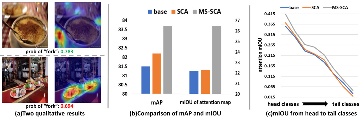
Figure 1: (a) The attention maps of two examples in MS-COCO (Lin et al., 2014) using ResNet $.01+\mathrm{SCA}$ (our baseline attention). (b) The mAP and attention map mIOU of ResNet101 baseline, SCA, and the MS-SCA (our de-confounded model). (c) Attention map mIOU of the three models from head classes to tail classes.
图 1: (a) 使用 ResNet $0.1+\mathrm{SCA}$ (我们的基线注意力) 在 MS-COCO (Lin et al., 2014) 中两个示例的注意力图。(b) ResNet101 基线、SCA 和 MS-SCA (我们的去混杂模型) 的 mAP 和注意力图 mIOU。(c) 从头部类别到尾部类别,三种模型的注意力图 mIOU。
To tackle the con founders in visual tasks, a common method is the causal intervention (Pearl et al., 2000; Neuberg, 2003). The interventions in most existing methods (Wang et al., 2021; Yang et al., 2021b; Yue et al., 2020; Zhang et al., 2020) share a maturity pipeline: defining the causality among given elements, implementing the con founders and ultimately implementing the backdoor adjustment (Pearl, 2014). Most of these methods, however, are difficult to implement on attention mechanism and migrate among different tasks. In this paper, we prove that a simple weighted multisampling operation on attention can be viewed as the intervention for the attention and confounding context. Based on that, we develop a novel causal attention module: Interventional Dual Attention (IDA). We first employ spatial class-aware attention (SCA) to extract the class-specific information in different positions of the feature map. Then, a multiple-sampling operation with Dot-Product Attention (DPA) re-weighting is implemented upon the SCA, which is essentially the causal intervention and builds a more robust attention map insensitive to the contextual bias. To receive a better trade-off between the performance and computation, we have two versions of IDA: the light one (pure two layers of attention) achieves huge improvements with limited parameter increment; the heavy one (the DPA is extended as a transformer) obtains the state-of-the-arts results with lower computation compared with the popular transformer-based models on the multi-label classification task. Furthermore, improvements in both classification and detection demonstrate the potential of our method to be applied in general visual tasks.
为解决视觉任务中的混杂因素,一种常见方法是因果干预 (Pearl et al., 2000; Neuberg, 2003)。现有大多数方法 (Wang et al., 2021; Yang et al., 2021b; Yue et al., 2020; Zhang et al., 2020) 的干预流程具有共性:先定义给定元素间的因果关系,再实施混杂因素控制,最终执行后门调整 (Pearl, 2014)。然而这些方法大多难以在注意力机制上实现,也难以跨任务迁移。本文证明,对注意力进行简单的加权多重采样操作可视为对注意力与混杂上下文的干预。基于此,我们开发了新型因果注意力模块:干预式双重注意力 (IDA)。首先采用空间类别感知注意力 (SCA) 提取特征图不同位置的类别特定信息,随后在SCA基础上实施带点积注意力 (DPA) 重加权的多重采样操作——该操作本质上是因果干预,能构建对上下文偏置不敏感的鲁棒注意力图。为平衡性能与计算开销,我们设计了两种IDA版本:轻量版 (纯双层注意力结构) 以有限参数增长实现显著性能提升;重量版 (将DPA扩展为Transformer结构) 在多标签分类任务中,相比主流基于Transformer的模型能以更低计算量取得最优结果。分类与检测任务的双重提升表明该方法在通用视觉任务中的应用潜力。
Our main contributions can be summarized as follows:
我们的主要贡献可概括如下:
2 RELATED WORK
2 相关工作
Attention Mechanism. Attention mechanism (Itti et al., 1998; Rensink, 2000; Corbetta & Shulman, 2002) aims at imitating the perception system of humans, which adopts sequence signals and selects to focus on salient parts. Hence, no matter in what forms, attention is expected to bias the weight towards the most informative parts of an input signal, and the signal can be varied from a sequence, feature map, or token queries in different tasks.
注意力机制 (Attention Mechanism)。注意力机制 (Itti et al., 1998; Rensink, 2000; Corbetta & Shulman, 2002) 旨在模仿人类的感知系统,通过处理序列信号并选择关注显著部分。因此,无论以何种形式实现,注意力机制都会将权重偏向输入信号中最具信息量的部分,而该信号在不同任务中可能表现为序列、特征图或token查询等形式。
Over the past several years, attention mechanism has won huge success in a wide range of tasks in computer vision. At the early stage, most of the works apply the attention to sequence-based models and tasks (Bluche, 2016; Stollenga et al., 2014). Then, here comes the age of attention is all your need (Vaswani et al., 2017), and many classic attention structures in computer vision arise such as SENET (Hu et al., 2018), Non-local (Wang et al., 2018) and CBAM (Woo et al., 2018). Finally is the popularity of self-attention (Do sov it ski y et al., 2020; Liu et al., 2021; Yuan et al., 2021) in these years, and it can be concluded as the operation among the query, key and value, which even totally replaces the CNN in pure visual tasks. However, as mentioned above, the usage of attention is usually not explicitly supervised. Consequently, the weight of attention is easily biased towards the bias in the dataset.
过去几年,注意力机制在计算机视觉的广泛任务中取得了巨大成功。早期大多数工作将注意力应用于基于序列的模型和任务 (Bluche, 2016; Stollenga et al., 2014)。随后进入《Attention Is All You Need》(Vaswani et al., 2017) 时代,涌现出SENET (Hu et al., 2018)、Non-local (Wang et al., 2018) 和CBAM (Woo et al., 2018) 等经典视觉注意力结构。近年来则是自注意力 (Dosovitskiy et al., 2020; Liu et al., 2021; Yuan et al., 2021) 的盛行,其本质可归结为查询(query)、键(key) 和值(value) 之间的运算,甚至在纯视觉任务中完全取代了CNN。但如前所述,注意力的使用通常缺乏显式监督,导致注意力权重容易偏向数据集中的偏差。
Causalities in Computer Vision. Causality is one of the most important research areas in machine learning including causal discovery (Yehezkel Rohekar et al., 2021; $\mathrm{Ng}$ et al., 2021), causal structure learning (Kivva et al., 2021; Akbari et al., 2021) and causal inference (Zhang et al., 2021; Kaddour et al., 2021). Recent years have also witnessed growing applications of causalities in visual tasks such as long-tail classification (Tang et al., 2020; Zhu et al., 2022), few/zero-shot learning (Yue et al., 2020; 2021), and Visual Question Answering (Chen et al., 2020; Niu et al., 2021; Yang et al., 2021a). Significantly, many of these works are about conquering the contextual bias in their tasks. Yue et al. (2020) considered pre-training information as the culprit for the bias and debiased by implementing the backdoor adjustment. Niu et al. (2021) clarified the “good” and “bad” language context and eliminated the bias by pursuing counter factual total causal effect.
计算机视觉中的因果关系。因果关系是机器学习中最重要的研究领域之一,包括因果发现 (Yehezkel Rohekar et al., 2021; $\mathrm{Ng}$ et al., 2021)、因果结构学习 (Kivva et al., 2021; Akbari et al., 2021) 和因果推断 (Zhang et al., 2021; Kaddour et al., 2021)。近年来,因果关系在视觉任务中的应用也日益增多,例如长尾分类 (Tang et al., 2020; Zhu et al., 2022)、少样本/零样本学习 (Yue et al., 2020; 2021) 和视觉问答 (Chen et al., 2020; Niu et al., 2021; Yang et al., 2021a)。值得注意的是,这些研究大多致力于克服任务中的上下文偏差。Yue et al. (2020) 将预训练信息视为偏差的根源,并通过实施后门调整来消除偏差。Niu et al. (2021) 区分了“好”与“坏”的语言上下文,并通过追求反事实总因果效应来消除偏差。
Most similar to our work, Yang et al. (2021b) and Wang et al. (2021) also visited the issue of attention aggravating the bias. Yang dealt with the confounding effect in vision-language tasks, and Wang resolved to build a more robust attention in OOD settings. However, our IDA is inherently different, especially with Wang et al. (2021) in two respects: 1) Different methods: we steer by the implementation of the confounder and other components when approximating the intervention, while Wang et al. (2021) focusing on the partition and annotation of each confounder explicitly. 2) Different applications: Wang et al. (2021) was aimed at OOD settings, which is a direct task for contextual debiasing, but lacks flexibility due to the requirement of pre-defining or clustering each context. In contrast, our model does not have as many limitations, and thus has the potential to be applied in more areas. Furthermore, Wang et al. (2021) has two defects: being evaluated in limited foregrounds and backgrounds (only animals in $I0$ contexts in NICO) and performing poorly when there are multiple objects. The two points are particularly attended to in our method because our model works well in full large-scale datasets of multi-label classification and detection.
与我们工作最为相似的是,Yang等人 (2021b) 和Wang等人 (2021) 也研究了注意力加剧偏差的问题。Yang处理了视觉语言任务中的混杂效应,而Wang致力于在OOD (Out-of-Distribution) 设置中构建更稳健的注意力机制。然而,我们的IDA (Intervention-based Debiased Attention) 在本质上有所不同,特别是与Wang等人 (2021) 在两个方面存在差异:1) 方法不同:我们在近似干预时通过混杂因子和其他组件的实现来引导,而Wang等人 (2021) 则明确关注每个混杂因子的划分和标注。2) 应用场景不同:Wang等人 (2021) 针对OOD设置,这是上下文去偏的直接任务,但由于需要预定义或聚类每个上下文而缺乏灵活性。相比之下,我们的模型没有那么多限制,因此有潜力应用于更多领域。此外,Wang等人 (2021) 存在两个缺陷:在有限的前景和背景中进行评估 (仅在NICO数据集的 $I0$ 上下文中使用动物) ,以及在存在多个对象时表现不佳。这两点在我们的方法中得到了特别关注,因为我们的模型在多标签分类和检测的大规模数据集中表现良好。
3 PRELIMINARIES: CAUSALITIES IN CONTEXTUAL BIAS
3 基础概念:上下文偏见中的因果关系
In this section, we first demonstrate a causal view of contextual bias in visual recognition. As is conveyed in Fig.2(a), we set up a simple Structural Causal Model (SCM), which clarifies the causality among the context $(C)$ , image content $(X)$ and the prediction $(Y)$ . In SCM, each link denotes causalities between two entities, e.g., $X\rightarrow Y$ means effect $Y$ is generated from $X$ . Although the appearance of SCM describing the contextual bias may be different in different tasks (Yue et al., 2020; Zhang et al., 2020; Yang et al., 2021b; Wang et al., 2021), their essence is depicted in Fig.2(a): an extra element $(C)$ respectively points to a pair of the cause $(X)$ and effect $(Y)$ where we want to build a mapping. Next, we will explore the rationale behind the SCM in detail.
在本节中,我们首先展示视觉识别中上下文偏见的因果视角。如图2(a)所示,我们建立了一个简单的结构因果模型(SCM),阐明了上下文$(C)$、图像内容$(X)$和预测结果$(Y)$之间的因果关系。在SCM中,每条连线表示两个实体间的因果关系,例如$X\rightarrow Y$表示效应$Y$由$X$产生。尽管描述上下文偏见的SCM表现形式可能因任务而异[20][21][22][23],但其本质如图2(a)所示:一个额外元素$(C)$分别指向我们希望建立映射关系的成因$(X)$和效应$(Y)$。接下来,我们将详细探讨该SCM背后的原理。
$X\rightarrow Y$ denotes the predictions depend on the content in images, which is the desired causal effect: to learn a network mapping an image to its prediction. The prediction is unbiased if the target in $X$ is the only causal relation between $X$ and $Y$ . $C\rightarrow X$ means the context prior determines how an image is constructed by the contents. For example, if all spoons in a dataset appear on the dining table, the dining table may be regarded as a necessary context when picturing the image of spoon. $C\rightarrow Y$ exists because the contextual information has a considerable impact on the prediction, i.e., the object itself and its context both affect the recognition of it. $X\leftarrow C\rightarrow Y$ together gives rise to a confounding effect: the network will be fooled into building a spurious causal relation e.g., dining table is taken as the cause for the prediction of spoon. Fig.2(b) further illustrates the role of attention. The attention module can not identify the confounding effect, but focus on intensifying the causal effect $X\rightarrow Y$ even if this causal link is wrong, causing the deterioration of context bias.
$X\rightarrow Y$ 表示预测依赖于图像中的内容,这是期望的因果效应:学习一个将图像映射到其预测的网络。如果 $X$ 中的目标是 $X$ 和 $Y$ 之间唯一的因果关系,则预测是无偏的。 $C\rightarrow X$ 表示上下文先验决定了图像如何由内容构建。例如,如果数据集中所有勺子都出现在餐桌上,餐桌可能被视为拍摄勺子图像时的必要背景。 $C\rightarrow Y$ 存在是因为上下文信息对预测有显著影响,即物体本身及其背景都会影响其识别。 $X\leftarrow C\rightarrow Y$ 共同产生了混杂效应:网络会被误导建立虚假的因果关系,例如将餐桌视为预测勺子的原因。图 2(b) 进一步说明了注意力的作用。注意力模块无法识别混杂效应,而是专注于强化因果效应 $X\rightarrow Y$,即使这种因果关系是错误的,从而导致上下文偏差的恶化。
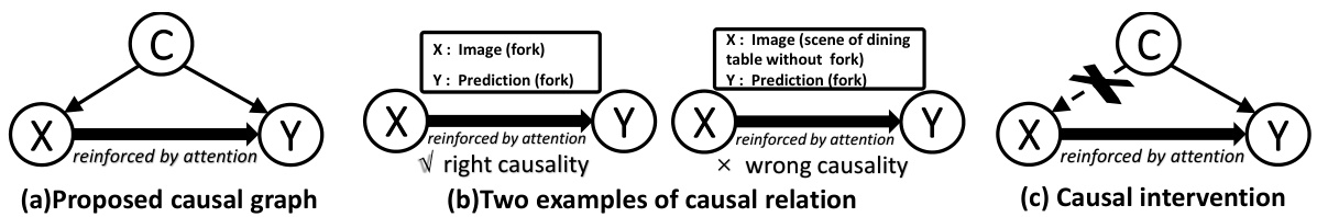
Figure 2: (a) The proposed causal graph for the causalities in contextual bias. (b) Two concrete causal examples. (c) The schematic diagram of causal intervention.
图 2: (a) 针对上下文偏差因果性提出的因果图。(b) 两个具体因果实例。(c) 因果干预示意图。
The sole way to eliminate the confounder is by causal intervention. The operation preserves the unavoidable context prediction $C\rightarrow Y$ and cuts off the bad link that an object relies on certain context. Common approaches to realizing intervention include RCT, frontdoor adjustment and backdoor adjustment (Pearl, 2014), while backdoor adjustment is the most frequently used in computer vision:
消除混杂因子的唯一方法是进行因果干预。该操作保留了不可避免的上下文预测 $C\rightarrow Y$ ,同时切断了物体依赖特定上下文的不良关联。实现干预的常用方法包括随机对照试验 (RCT) 、前门调整和后门调整 (Pearl, 2014) ,其中后门调整在计算机视觉领域应用最为广泛:
$$
\mathrm{P}(Y|\mathrm{do}(X))=\sum_{c}\mathrm{P}(Y|X,C=c)\mathrm{P}(C=c),
$$
$$
\mathrm{P}(Y|\mathrm{do}(X))=\sum_{c}\mathrm{P}(Y|X,C=c)\mathrm{P}(C=c),
$$
where the do-operation denotes the causal intervention cutting off the edge $C\rightarrow X$ as illustrated in Fig.2(c). Free from the interference of confounding path, the network can always learn the unbiased causality between $X$ and $Y$ . Here, $X$ can be extended as attention features. Consequently, the reinforcement from the attention mechanism can lead to a better prediction.
其中do操作表示因果干预切断边 $C\rightarrow X$ ,如图2(c)所示。摆脱混杂路径的干扰后,网络总能学习到 $X$ 和 $Y$ 之间的无偏因果关系。此处 $X$ 可扩展为注意力特征。因此,注意力机制的强化能带来更好的预测效果。
4 METHODOLOGY
4 方法论
In this section, we present a novel framework that strengthens the robustness of attention on contextual bias. The overview of our model is illustrated in Fig.3. We first introduce our baseline attention: Spatial Class-Aware Attention (SCA), which can obtain class-specific representations but need guidance (Section 4.1). Then, to guarantee the attention module emphasizes the proper causality, we deduce and migrate the backdoor adjustment for the attention, where the intervention is approximated as the multiple sampling with re-weighting upon SCA (Section 4.2). Finally, we present the concrete implementation in our method, i.e., implementing three versions of multiple sampling on SCA (MS-SCA) and implementing the re-weighting as Dot-Product Attention (DPA) or the transformer (Section 4.3).
在本节中,我们提出了一种增强上下文偏置注意力鲁棒性的新框架。模型概览如图3所示。首先介绍基线注意力机制:空间类感知注意力 (SCA) ,它能获取类特定表征但需要引导 (第4.1节) 。接着,为确保注意力模块聚焦正确的因果关系,我们推导并迁移了注意力的后门调整方法,通过SCA的多重采样与重加权来近似干预 (第4.2节) 。最后展示具体实现方案:在SCA上实现三重采样变体 (MS-SCA) ,并将重加权实现为点积注意力 (DPA) 或Transformer (第4.3节) 。
4.1 CLASS-AWARE LAYER
4.1 类别感知层
The target of our Spatial Class-Aware Attention (SCA) is to bias the spatial representations toward where the objects are the most likely to show up for each category. Given an image, we can obtain its feature map $\mathbf{X}\in\mathbb{R}^{H\times W\times D}$ from either a CNN-based or a transformer-based backbone, where $D,H,W$ denotes the channel dimension, height, and width. Our purpose is to turn $\mathbf{X}$ into a categoryaware representations $\mathbf{E}={\mathbf{e}{k}}{k=1}^{K}\in\mathbb{R}^{K\times D}$ , where $K$ is the number of the classes. For each specific class $k$ , its representation $\mathbf{e}_{k}$ is computed from the weighted average of the spatial feature in $\mathbf{X}$ . Then, the feature for each category can be reformed according to its unique spatial information:
我们的空间类别感知注意力 (Spatial Class-Aware Attention, SCA) 的目标是让空间表征偏向于每个类别最可能出现物体的区域。给定一张图像,我们可以从基于 CNN 或基于 Transformer 的主干网络中获取其特征图 $\mathbf{X}\in\mathbb{R}^{H\times W\times D}$ ,其中 $D,H,W$ 分别表示通道维度、高度和宽度。我们的目的是将 $\mathbf{X}$ 转换为类别感知表征 $\mathbf{E}={\mathbf{e}{k}}{k=1}^{K}\in\mathbb{R}^{K\times D}$ ,其中 $K$ 是类别数量。对于每个特定类别 $k$ ,其表征 $\mathbf{e}_{k}$ 是通过对 $\mathbf{X}$ 中的空间特征进行加权平均计算得到的。这样,每个类别的特征可以根据其独特的空间信息进行重构:
$$
\mathbf{e}{k}=\sum_{i=1}^{H}\sum_{j=1}^{W}\operatorname{P}(Y=k|X=x_{i,j})x_{i,j},
$$
$$
\mathbf{e}{k}=\sum_{i=1}^{H}\sum_{j=1}^{W}\operatorname{P}(Y=k|X=x_{i,j})x_{i,j},
$$
where $\mathrm{P}(Y=k|X=x_{i,j})$ is obtained by feeding $x_{i,j}$ into a linear classifier $\mathrm{f^{clf}}\left(.\right)$ followed with a softmax $(.)$ regular iz ation.
其中 $\mathrm{P}(Y=k|X=x_{i,j})$ 是通过将 $x_{i,j}$ 输入线性分类器 $\mathrm{f^{clf}}\left(.\right)$ 再经过 softmax $(.)$ 归一化得到的。
We adopt SCA as our baseline attention for two reasons: 1) SCA is useful for multi-object tasks. 2) SCA is easier to be affected by contextual bias (Zhu et al., 2017a; Ye et al., 2020; Zhao et al., 2021). Quite a few works adopt similar class-specific representations, due to the insight and interpret ability that they empower the models to capture object-aware features in different areas of different images, which is significant for multi-instance tasks. However, pure SCA works badly because it needs guidance to capture causal locations. SCA is designed to underline crucial positions for each class, while the “crucial position” could be the familiar background due to the bias in the dataset. To tackle this problem, other works mainly employ complicated structures (e.g., GCN or Transformer) to further process the representations. By contrast, we argue that a simple intervention (Sec.4.2) is enough to inspire the potentiality of class-aware attention. In the appendix A.4, we show our framework also gains improvement on other classic attention structures.
我们采用SCA作为基线注意力机制的原因有二:1) SCA适用于多目标任务;2) SCA更容易受到上下文偏差的影响 (Zhu et al., 2017a; Ye et al., 2020; Zhao et al., 2021)。许多工作采用类似的类别特定表示方法,因为它们能赋予模型捕捉不同图像区域中物体感知特征的能力,这对多实例任务至关重要。然而纯SCA效果不佳,因为它需要引导才能捕捉因果位置。SCA的设计初衷是突出每个类别的关键位置,但由于数据集偏差,这些"关键位置"可能是熟悉的背景。为解决这个问题,其他工作主要采用复杂结构(如GCN或Transformer)进一步处理表示。相比之下,我们认为简单干预(第4.2节)就足以激发类别感知注意力的潜力。附录A.4显示我们的框架在其他经典注意力结构上也能获得改进。
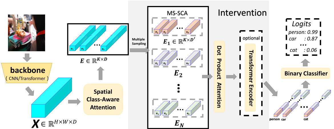
Figure 3: Overview of our proposed model. $X$ could be either image feature from visual backbone or ROI feature from detection backbone. The model is composed of the baseline attention (SCA), the multiple sampling on SCA (MS-SCA), and the second attention layer (DPA or transformer).
图 3: 我们提出的模型概览。$X$ 可以是视觉主干网络提取的图像特征,也可以是检测主干网络提取的 ROI 特征。该模型由基线注意力 (SCA)、SCA 多重采样 (MS-SCA) 和第二注意力层 (DPA 或 Transformer) 组成。
4.2 CAUSAL INTERVENTION
4.2 因果干预
$\operatorname{P}(Y|\mathrm{do}(X=x))$ calculates the probability of $Y$ when all $X$ turns to $x$ , which is infeasible. Thereby, backdoor adjustment indeed uses realistic statistics (without $d o$ ) to attain the effect equivalent to do-operation. However, it is still challenging that we are required to stratify and sample every possible $c$ for rigorous backdoor adjustment in Eq. 1. In practice, it’s difficult to quant if i cat every possible context, and consequently the $\mathrm{P}(C=c)$ is not explicitly observable.
$\operatorname{P}(Y|\mathrm{do}(X=x))$ 计算当所有 $X$ 变为 $x$ 时 $Y$ 的概率,这是不可行的。因此,后门调整 (backdoor adjustment) 实际上使用现实统计量(不含 $do$ 运算)来达到与干预操作等效的效果。然而,挑战在于我们需要对每个可能的 $c$ 进行分层采样才能严格满足公式 1 的后门调整要求。实践中很难量化所有可能的上下文 (context) ,因此 $\mathrm{P}(C=c)$ 无法显式观测到。
Thanks to the perspective of Inverse Probability Weighting (IPW) (Pearl, 2009), which further reforms the adjustment and simplifies the implementation, we can approximate the sampling on $c$ via the sampling on the observed data, i.e., $(k,x)$ . Firstly, we rewrite Eq. 1 to get the equivalent formula:
得益于逆概率加权 (Inverse Probability Weighting, IPW) (Pearl, 2009) 的视角,它进一步改进了调整方法并简化了实现,我们可以通过观测数据 $(k,x)$ 上的采样来近似 $c$ 上的采样。首先,我们将公式 1 重写为等价形式:
$$
\begin{array}{l}{{\displaystyle\mathrm{P}(Y=k|\mathrm{d}\mathrm{o}(X=x))=\sum_{c}\frac{\mathrm{P}(Y=k,X=x|C=c)\mathrm{P}(C=c)}{\mathrm{P}(X=x|C=c)}.}}\ {{\displaystyle=\sum_{c}\frac{\mathrm{P}(Y=k,X=x,C=c)}{\mathrm{P}(X=x|C=c)},}}\end{array}
$$
$$
\begin{array}{l}{{\displaystyle\mathrm{P}(Y=k|\mathrm{d}\mathrm{o}(X=x))=\sum_{c}\frac{\mathrm{P}(Y=k,X=x|C=c)\mathrm{P}(C=c)}{\mathrm{P}(X=x|C=c)}.}}\ {{\displaystyle=\sum_{c}\frac{\mathrm{P}(Y=k,X=x,C=c)}{\mathrm{P}(X=x|C=c)},}}\end{array}
$$
where $1/\mathrm{P}(X=x|C=c)$ is the so-called inverse weight. Although it’s hard to sample $c$ , in Eq. 4, there is only one $(k,x)$ given one $c$ , thereby, the number of $c$ that Eq. 4 would encounter equals the number of samples $(k,x)$ we observe. As a result, the observed $\mathrm{P}(Y,X,C)$ can be used to approximate $\operatorname{P}(Y=k|\mathrm{do}(X=x))$ , i.e., the essence of IPW lies in “assign the Inverse Weight $1/\bar{\mathrm{P}(X=x|C=c)}$ to every observed $\mathrm{P}(Y,X,C)$ , and act as though they were drawn from the post-intervention $\operatorname{P}(Y=k|\mathrm{do}(X=x))^{,}$ (Pearl, 2009). Hence, Eq. 4 can be further approximated as:
其中 $1/\mathrm{P}(X=x|C=c)$ 是所谓的逆概率权重。尽管难以对 $c$ 进行采样,但在公式4中,给定一个 $c$ 时仅存在一个 $(k,x)$ ,因此公式4会遇到的 $c$ 数量等于我们观察到的样本 $(k,x)$ 数量。于是,观测到的 $\mathrm{P}(Y,X,C)$ 可用于近似 $\operatorname{P}(Y=k|\mathrm{do}(X=x))$ ,即IPW的核心思想在于"为每个观测到的 $\mathrm{P}(Y,X,C)$ 分配逆权重 $1/\bar{\mathrm{P}(X=x|C=c)}$ ,并视作它们来自干预后的 $\operatorname{P}(Y=k|\mathrm{do}(X=x))^{,}$" (Pearl, 2009)。因此,公式4可进一步近似为:
$$
\operatorname{P}\left(Y=k|\operatorname{do}(X=x)\right)\approx\sum_{n=1}^{N}{\frac{\operatorname{P}(Y=k,X=x^{n},C=c)}{\operatorname{P}(X=x^{n}|C=c)}},
$$
$$
\operatorname{P}\left(Y=k|\operatorname{do}(X=x)\right)\approx\sum_{n=1}^{N}{\frac{\operatorname{P}(Y=k,X=x^{n},C=c)}{\operatorname{P}(X=x^{n}|C=c)}},
$$
which transforms the summation of $\mathrm{^C}$ into the sampling of X, and $\mathbf{N}$ is sampling times. Here, $C$ in the numerator can be omitted following the common practice of IPW. Then, we model terms in the summation as the sigmoid activated classification probability of the class-aware attention features :
将 $\mathrm{^C}$ 的求和转化为对 X 的采样,其中 $\mathbf{N}$ 为采样次数。根据逆概率加权 (IPW) 的常规做法,分子中的 $C$ 可省略。随后,我们将求和项建模为类别感知注意力特征经 sigmoid 激活后的分类概率:
$$
\mathrm{P}(Y=k|\mathrm{do}(X=x))=\sum_{n=1}^{N}{\frac{\mathrm{P}(Y=k|X=x^{n})\mathrm{P}(X=x^{n})}{\mathrm{P}(X=x^{n}|C=c)}}=\sum_{n=1}^{N}{\frac{\mathrm{Sigmoid}(w_{k}e_{k}^{n})\mathrm{P}(e_{k}^{n})}{\mathrm{P}(X=e_{k}^{n}|C=c)}}
$$
$$
\mathrm{P}(Y=k|\mathrm{do}(X=x))=\sum_{n=1}^{N}{\frac{\mathrm{P}(Y=k|X=x^{n})\mathrm{P}(X=x^{n})}{\mathrm{P}(X=x^{n}|C=c)}}=\sum_{n=1}^{N}{\frac{\mathrm{Sigmoid}(w_{k}e_{k}^{n})\mathrm{P}(e_{k}^{n})}{\mathrm{P}(X=e_{k}^{n}|C=c)}}
$$
where $w_{k}$ is the classifier weight for class $\mathrm{k\Omega}$ and $e_{k}$ is the feature of class $\mathrm{k\Omega}$ in Sec. 4.1. Meanwhile, the denominator, $i.e.$ , the inverse weight, can be the Propensity Score (Austin, 2011) in the classification model following Rubin’s theory, where the normalization effect is divided into the treated
其中 $w_{k}$ 是类别 $\mathrm{k\Omega}$ 的分类器权重,$e_{k}$ 是第4.1节中类别 $\mathrm{k\Omega}$ 的特征。同时,分母(即逆权重)可以是分类模型中遵循Rubin理论的倾向得分 (Propensity Score) (Austin, 2011),其中归一化效应被划分为处理组
class-specific group $(|w_{k}|{2}\cdot|e_{k}^{n}|{2})$ and untreated class-agnostic group $(\gamma\cdot|e_{k}^{n}|{2})$ . Moreover, the confounder (context) in our model is countable, thereby the sampled $e_{k}^{n}$ is finite and we simplify the $|e_{k}^{n}|_{2}$ as 1. Finally, we compute the ultimate intervention effect by assembling them as follows:
特定类别组 $(|w_{k}|{2}\cdot|e_{k}^{n}|{2})$ 和未处理的类别无关组 $(\gamma\cdot|e_{k}^{n}|{2})$ 。此外,我们模型中的混杂因素(上下文)是可数的,因此采样的 $e_{k}^{n}$ 是有限的,并将 $|e_{k}^{n}|_{2}$ 简化为1。最终,我们通过如下方式组合计算最终的干预效果:
$$
\operatorname{P}(Y=k|\mathrm{d}\boldsymbol{0}(X=x))=\sum_{n=1}^{N}{\frac{\mathrm{Sigmoid}(w_{k}e_{k}^{n})}{|w_{k}|{2}+\gamma}}\mathrm{P}(e_{k}^{n}),
$$
$$
\operatorname{P}(Y=k|\mathrm{d}\boldsymbol{0}(X=x))=\sum_{n=1}^{N}{\frac{\mathrm{Sigmoid}(w_{k}e_{k}^{n})}{|w_{k}|{2}+\gamma}}\mathrm{P}(e_{k}^{n}),
$$
where the implementations of $e^{n}$ and $\mathrm{P}(e_{k}^{n})$ are unfolded in the next section. In Sec.5.3, we will show that the SCA with multiple sampling intervention makes up a $\mathrm{{}^{\cdot\leftarrow}1+1>2^{\prime\prime}}$ effect.
其中 $e^{n}$ 和 $\mathrm{P}(e_{k}^{n})$ 的具体实现将在下一节展开。在5.3节中,我们将证明采用多重采样干预的SCA能产生 $\mathrm{{}^{\cdot\leftarrow}1+1>2^{\prime\prime}}$ 效应。
4.3 SAMPLING AND RE-WEIGHTING LAYER
4.3 采样与重加权层
In Eq. 7, the multiple sampling on $e_{k}$ is crucial to the intervention on the attention. Next, given a fixed feature dimension and sampling dimension (e.g., 2048 and 512), we describe several versions of multiple sampling on SCA (MS-SCA): 1) Random sampling: complete randomness is of no mean and unfriendly to back propagation, hence, we assign random starting points and random intervals for each sample, and the interval for a single sample is fixed. 2) Multi-head (Vaswani et al., 2017): we equally divide the channel into $\mathbf{N}$ groups and take each group as a sample. 3) Channel-shuffle: considering the success of Pixel Shuffle (Shi et al., 2016; Liu et al., 2021), the shuffle on the channel may also be meaningful. In fact, the multi-head operation is a Channel-shuffle with interval 1. Moreover, channel-shuffle can boost the sampling times with different assigned intervals. Interestingly, we will show by experiments that our model is not sensitive to these choices, indicating that the generic multi-sampling behavior is the main reason for the observed improvements.
在公式7中,对 $e_{k}$ 的多重采样是注意力干预的关键。接下来,在给定固定特征维度和采样维度(例如2048和512)的情况下,我们描述了SCA (MS-SCA) 多重采样的几种实现方式:
- 随机采样:完全随机性缺乏意义且不利于反向传播,因此我们为每个样本分配随机起始点和随机间隔,单个样本的间隔保持固定。
- 多头机制 (Vaswani et al., 2017) :将通道均匀划分为 $\mathbf{N}$ 组,每组视为一个样本。
- 通道混洗:受Pixel Shuffle (Shi et al., 2016; Liu et al., 2021) 成功的启发,通道混洗可能同样有效。实际上,多头操作是间隔为1的通道混洗特例。此外,通道混洗可通过不同间隔设置提升采样次数。有趣的是,实验将表明我们的模型对这些选择并不敏感,说明通用的多重采样行为才是性能提升的主因。
Finally is the implementation of $\mathrm{P}(e_{k}^{n})$ . The simplest way is to assign $\mathrm{P}(e_{k}^{n})$ as $1/N$ , which assumes a uniform prior of each sample. However, the status of each sample is unequal. Different positions in channel-wise dimension attend to different objects (Zhu et al., 2017b), hence, to achieve better class-aware features, it is necessary to bias the weight into the more crucial samples rather than the average. Another alternative is to introduce the learnable re-weight parameters, nonetheless, the learning capacity is limited and it is hard to scale up the model.
最后是实现 $\mathrm{P}(e_{k}^{n})$ 的方法。最简单的方式是将 $\mathrm{P}(e_{k}^{n})$ 设为 $1/N$ ,即假设每个样本具有均匀先验。然而,每个样本的状态并不平等。通道维度上的不同位置关注不同对象 (Zhu et al., 2017b) ,因此为了获得更好的类感知特征,需要将权重偏向更关键的样本而非平均分配。另一种方案是引入可学习的重加权参数,但其学习能力有限且难以扩展模型规模。
In consequence, we adopt another attention to operate the re-weighting. After the multiple sampling, we get sample-specific class-aware feature $\mathbf{E}\in\mathbb{R}^{B\times N\times K\times D^{\prime}}$ , where $B$ denotes the batch size and $D^{\prime}$ is sampling dimension. Then, we resize $\mathbf{E}$ into the sequence $\mathbf{E}^{s}\in\mathbb{R}^{N\times(B*K)\times D^{\prime}}$ . Now, we can implement the scaled Dot-Product Attention (Vaswani et al., 2017) (DPA) to re-weight among different samples, for each class-aware representation:
因此,我们采用另一种注意力机制进行重新加权。经过多次采样后,我们得到样本特定的类感知特征 $\mathbf{E}\in\mathbb{R}^{B\times N\times K\times D^{\prime}}$ ,其中 $B$ 表示批次大小, $D^{\prime}$ 为采样维度。随后,我们将 $\mathbf{E}$ 调整为序列形式 $\mathbf{E}^{s}\in\mathbb{R}^{N\times(B*K)\times D^{\prime}}$ 。此时,我们可以对每个类感知表征实施缩放点积注意力 (Vaswani et al., 2017) (DPA) 来实现样本间的重新加权:
$$
\mathbf{E^{\delta^{\prime}}}=\operatorname{softmax}(\frac{(W_{q}\mathbf{E}^{s})(W_{k}\mathbf{E}^{s})^{T}}{\sqrt{D^{\prime}}})(W_{v}\mathbf{E}^{s}),
$$
$$
\mathbf{E^{\delta^{\prime}}}=\operatorname{softmax}(\frac{(W_{q}\mathbf{E}^{s})(W_{k}\mathbf{E}^{s})^{T}}{\sqrt{D^{\prime}}})(W_{v}\mathbf{E}^{s}),
$$
where $W_{q},W_{k},W_{v}$ are the linear projection mapping the sequence into a common subspace for similarity measure. Thus far, we have explained our lightweight version of IDA. Our method increases almost no parameter except the shared KQV projection, and it outperforms all other models with comparable computation. Furthermore, to scale up the model, Eq. 8 can be naturally extended as the transformer, providing opportunities to trade-off between computation and performance:
其中 $W_{q},W_{k},W_{v}$ 是将序列线性投影到公共子空间以进行相似度度量的矩阵。至此,我们已阐述了轻量级IDA (Iterative Deepening Attention) 的实现方案。该方法除共享的KQV (Key-Query-Value) 投影外几乎不增加参数,在计算量相当的情况下性能优于所有其他模型。此外,为扩展模型规模,公式8可自然扩展为Transformer架构,从而在计算量与性能之间实现灵活权衡:
$$
\mathbf{E}^{s+1}=\operatorname*{max}(0,\mathbf{E}^{s^{\prime}}W_{1}+b_{1})W_{2}+b_{2}.
$$
$$
\mathbf{E}^{s+1}=\operatorname*{max}(0,\mathbf{E}^{s^{\prime}}W_{1}+b_{1})W_{2}+b_{2}.
$$
Eq. 8 and Eq. 9 can continue iterating to build a stronger class-specific representation, which becomes our heavyweight version of IDA. Finally, the class-aware representations are fed into a binary classifier followed by a sigmoid activation, and the average logit of all samples is taken as the final logit for that class, where the classifier shares the same learnable weight with $\mathrm{f^{clf}}\left(.\right)$ in $\mathrm{Sec4.1}$ .
式8和式9可以继续迭代以构建更强的类特定表示,这成为我们的重量级IDA版本。最后,类感知表示被输入到一个二元分类器中,后接一个sigmoid激活函数,所有样本的平均logit作为该类的最终logit,其中分类器与$\mathrm{Sec4.1}$中的$\mathrm{f^{clf}}\left(.\right)$共享相同的可学习权重。
5 EXPERIMENTS
5 实验
In this section, we conduct extensive experiments to demonstrate the superiority of the proposed method. We first introduce the general settings. Then, we present our quantitative results of multilabel classification and detection on three widely used datasets: MS-COCO (Lin et al., 2014), VOC2007, and VOC2012 (Everingham et al., 2010). Finally, we perform various ablation studies and analyses to show the effectiveness of different components in our model.
在本节中,我们通过大量实验验证所提方法的优越性。首先介绍通用实验设置,随后在三个广泛使用的数据集(MS-COCO (Lin et al., 2014)、VOC2007和VOC2012 (Everingham et al., 2010))上展示多标签分类与检测的量化结果。最后通过消融实验与分析,验证模型中各组成部分的有效性。
Table 1: Comparison of mAP $(%)$ on the MS-COCO in multi-label classification. L and H mean the light version and the heavy version respectively, and WH denotes the resolution.
表 1: MS-COCO 多标签分类任务中 mAP (%) 的对比。L 和 H 分别表示轻量版和重量版,WH 表示分辨率。
| 方法 | 分辨率 | mAP | All | All | Top3 | Top3 |
|---|---|---|---|---|---|---|
| CF1 | OF1 | CF1 | OF1 | |||
| ResNet-101 (He et al., 2016) | 448 * 448 | 81.5 | 76.3 | 80.0 | 73.5 | 76.0 |
| ML-GCN (Chen et al., 2019c) | 448 * 448 | 83.0 | 78.0 | 80.3 | 74.2 | 76.3 |
| MS-CMA (You et al., 2020) | 448 * 448 | 83.8 | 78.4 | 81.0 | 74.9 | 77.1 |
| CSRA (Zhu & Wu, 2021) | 448 * 448 | 83.5 | 77.9 | 80.3 | 74.4 | 76.5 |
| IDA-R101(L) | 448 * 448 | 84.3 | 78.5 | 81.1 | 73.6 | 77.3 |
| IDA-R101(H) | 448 * 448 | 84.8 | 78.7 | 80.9 | 73.9 | 77.4 |
| SSGRL (Chen et al., 2019b) | 576 * 576 | 83.8 | 76.8 | 79.7 | 72.7 | 76.2 |
| C-Trans (Lanchantin et al., 2021) | 576 * 576 | 85.1 | 79.9 | 81.7 | 76.0 | 77.6 |
| ADD-GCN (Ye et al., 2020) | 576 * 576 | 85.2 | 80.1 | 82.0 | 75.8 | 77.9 |
| CCD (Liu et al., 2022) | 576 * 576 | 85.3 | 80.2 | 82.1 | 76.0 | 77.9 |
| TDRG (Zhao et al., 2021) | 576 * 576 | 86.0 | 80.4 | 82.4 | 76.2 | 78.1 |
| IDA-R101(L) | 576 * 576 | 85.5 | 79.8 | 82.3 | 75.2 | 78.1 |
| IDA-R101(H) | 576 * 576 | 86.3 | 80.4 | 82.5 | 76.4 | 78.2 |
| Swin-Base (Liu et al., 2021) | 384 * 384 | 88.4 | 82.2 | 84.0 | 77.2 | 79.9 |
| Swin-Large (Liu et al., 2021) | 384 * 384 | 89.3 | 83.6 | 85.6 | 78.1 | 80.8 |
| MA-SwinB(H) | 384 * 384 | 89.3 | 83.7 | 85.1 | 78.0 | 80.4 |
| IMA-SwinL(H) | 384 * 384 | 90.3 | 84.7 | 85.9 | 79.0 | 81.1 |
Table 2: Comparison of between our method and the baseline on the MS-COCO and VOC07 in object detection.
表 2: 我们的方法与基线在目标检测任务中 MS-COCO 和 VOC07 数据集上 的对比
| 方法 | 检测器 | MS-COCO mAP@.5 mAP@.75 | VOC07 mAP@.5 |
|---|---|---|---|
| 基线 | Faster-RCNN-ROIAlign-R50 | 58.1 | 40.5 |
| IDA (L) | Faster-RCNN-ROIAlign-R50 | 59.3 | 42.0 |
| IDA (L) | RetinaNet-R50 | 52.5 | 36.6 |
| 基线 IDA (L) | RetinaNet-R50 | 55.8 | 38.6 |
| 基线 IDA (L) | DeTR-DC5-R101 | 64.7 | 47.7 |
| 基线 IDA (L) | DeTR-DC5-R101 | 65.7 | 49.2 |
5.1 EXPERIMENTS SETTINGS
5.1 实验设置
Implementation details. Unless otherwise stated, we use ResNet101 (He et al., 2016) pre-trained on ImageNet 1k (Deng et al., 2009) as our backbone. For the multiple-sampling module, we adopt channel-shuffle with start point $=0$ , intervals $=1$ & 2, and sampling dimension $=512$ (1/4 of the full dimension), and thus we have $=8$ . $\gamma$ is set as 1/32. For the heavy version of IDA, we only have 2 layers of transformer and do not implement the multi-head operation on dot-product attention. There is no extra data preprocessing besides the standard data augmentation (Ridnik et al., 2021; Chen et al., 2019c). The multi-label classification model and the detection model are both optimized by the Binary Cross Entropy Loss with sigmoid. We choose Adam as our optimizer with weight decay of $1e-4$ and $(\beta_{1},\bar{\beta_{2}})=(0.9,0.9\bar{9}99)$ . The learning rate is $1e-4$ for the batch size of 128 with a 1-cycle policy. All our codes were implemented in Pytorch (Paszke et al., 2017).
实现细节。除非另有说明,我们使用在ImageNet 1k (Deng et al., 2009) 上预训练的ResNet101 (He et al., 2016) 作为主干网络。对于多重采样模块,我们采用通道混洗(channel-shuffle),起始点 $=0$,间隔 $=1$ 和 2,采样维度 $=512$ (全维度的1/4),因此得到 $=8$。$\gamma$ 设为1/32。在IDA的重度版本中,我们仅使用2层Transformer且未在点积注意力中实现多头操作。除标准数据增强(Ridnik et al., 2021; Chen et al., 2019c)外,未进行额外数据预处理。多标签分类模型和检测模型均采用带sigmoid的二值交叉熵损失进行优化。我们选择Adam作为优化器,权重衰减为 $1e-4$,$(\beta_{1},\bar{\beta_{2}})=(0.9,0.9\bar{9}99)$。学习率设为 $1e-4$,批量大小为128,采用1-cycle策略。所有代码均基于Pytorch (Paszke et al., 2017)实现。
Evaluation metrics. For multi-label classification, we adopt the mean average precision (mAP) as our main evaluation metric, and overall/per-class F1-measure (OF1/CF1) as supplements. Separate precision and recall are not employed because they are easily affected by the hyper-parameter. For detection, we employ the $\operatorname*{mAP}@.5$ , mAP $\ @.7$ 5 and mAP $@$ [.5, .95] for MS-COCO, and $\operatorname*{mAP}@.5$ for Pascal VOC. In Sec. 5.3, we also evaluate our method on contextual bias benchmarks. The result of classification on Pascal VOC can be found in Appendix A.1.
评估指标。对于多标签分类任务,我们采用平均精度均值 (mAP) 作为主要评估指标,并以整体/各类别 F1 值 (OF1/CF1) 作为补充指标。未单独采用精确率和召回率,因为它们容易受超参数影响。在检测任务中,我们对 MS-COCO 数据集使用 $\operatorname*{mAP}@.5$、mAP $\ @.7$ 5 和 mAP $@$ [.5, .95] 指标,对 Pascal VOC 数据集使用 $\operatorname*{mAP}@.5$ 指标。在 5.3 节中,我们还针对上下文偏置基准测试评估了本方法。Pascal VOC 上的分类结果详见附录 A.1。
5.2 QUANTITATIVE RESULTS.
5.2 定量结果
Multi-label classification on MS-COCO. MS-COCO (Lin et al., 2014) is the most popular benchmark for object detection, segmentation and caption, and has also become widely used in multi-label recognition recently. It contains 122,218 images and covers 80 categories with 2.9 for each image on average. Considering the result of multi-label classification is highly related to the resolution and backbone, we perform experiments with different backbones and different resolutions to make the result more persuasive.
MS-COCO上的多标签分类。MS-COCO (Lin et al., 2014) 是最流行的目标检测、分割和描述基准数据集,近年来也广泛应用于多标签识别领域。该数据集包含122,218张图像,涵盖80个类别,平均每张图像包含2.9个标签。考虑到多标签分类结果与图像分辨率和主干网络(backbone)高度相关,我们采用不同主干网络和分辨率进行实验以使结果更具说服力。
As is demonstrated in Table 1, for CNN backbone, we adopt ResNet101 pre-trained on ImageNet 1k with the resolutions of $448\times448$ and $576\times576$ . The results of lightweight and heavyweight versions are both present for fair comparisons. The first block shows that our light model has an obvious advantage over other methods with comparable computation (e.g., CSRA (Zhu & Wu, 2021)). For heavyweight models, other models universally adopt 3 or more layers of transformer or GNN (e.g., ADDGCN (Ye et al., 2020), C-Trans (Lanchantin et al., 2021) and TDRG (Zhao et al., 2021)), while ours only has two layers but outperforms all of them, confirming the trade-off between computation and performance in our method is more efficient. For transformer backbone, we use the recently popular Swin-Transformer (Liu et al., 2021) pre-trained on ImageNet $22\mathrm{k\Omega}$ . The results in the last block convey our improvement. Based on such a strong backbone, it is very difficult to advance the performance, but our method still brings about considerable progress. In Appendix A.2, we further present the comparison of FLOPs and parameters among some of these methods.
如表 1 所示,对于 CNN 主干网络,我们采用了在 ImageNet 1k 上预训练的 ResNet101,分辨率为 $448\times448$ 和 $576\times576$。为了公平比较,同时展示了轻量级和重量级版本的结果。第一组数据显示,在计算量相当的情况下(例如 CSRA (Zhu & Wu, 2021)),我们的轻量模型明显优于其他方法。对于重量级模型,其他方法普遍采用 3 层或更多层的 Transformer 或 GNN(例如 ADDGCN (Ye et al., 2020)、C-Trans (Lanchantin et al., 2021) 和 TDRG (Zhao et al., 2021)),而我们的模型仅有两层却表现更优,这证实了我们的方法在计算量与性能之间的权衡更为高效。对于 Transformer 主干网络,我们使用了近期流行的 Swin-Transformer (Liu et al., 2021),并在 ImageNet $22\mathrm{k\Omega}$ 上进行了预训练。最后一组数据展示了我们的改进效果。基于如此强大的主干网络,进一步提升性能非常困难,但我们的方法仍带来了显著进步。在附录 A.2 中,我们进一步对比了这些方法的 FLOPs 和参数量。
Table 3: Ablation studies on components of our method with different resolutions. DPA means the dot-product attention in the second layer and Trans means extending the DPA as a transformer.
表 3: 不同分辨率下我们方法各组成部分的消融研究。DPA表示第二层中的点积注意力 (dot-product attention),Trans表示将DPA扩展为Transformer。
| Components | mAP | ||||
|---|---|---|---|---|---|
| SCA | Multi-Sampling | DPA | Trans | 448*448 | 576*576 |
| 81.4 | 82.7 | ||||
| 81.9 | 83.0 | ||||
| √ | 82.1 | 83.0 | |||
| √ | 83.6 | 84.8 | |||
| √ | 82.2 | 83.1 | |||
| √ | 84.3 | 85.5 | |||
| √ | 人 | 84.8 | 86.3 |
Object Detection on MS-COCO and Pascal VOC. Our framework receives the feature map, which can also adopt the ROI features in bounding box as input. Therefore, our method can be seamlessly applied to the detection, including RCNN-like, YOLO-like and DETR-like methods whose neck output the feature maps. To validate that our method can gain improvement in a wider range of visual tasks, we also conduct experiments on object detection on the two widely used datasets. We employ the Faster-RCNN (Ren et al., 2015), RetinaNet (Lin et al., 2017), and DETR (Carion et al., 2020) as our basic detector. The IDA is directly implemented on the RoI feature maps from the neck and the original bbox head is reserved as the residual path which is different from the classification. All the code is implemented in mm detection (Chen et al., 2019a). The results are shown in Table2. We observe considerable improvements from the baseline on all detectors and datasets, revealing the generalization of IDA on other recognition tasks. Whereas, it must be admitted that the enhancement is not as significant as that in classification, because the role of IDA partly overlaps with the location module in the detection model. Hence, our method obtains greater improvements in the one-stage detection whose object regions are not as accurate as those in two-stage detection.
在MS-COCO和Pascal VOC上的目标检测。我们的框架接收特征图作为输入,也可以采用边界框中的ROI特征。因此,我们的方法可以无缝应用于包括类似RCNN、类似YOLO和类似DETR等输出特征图的检测方法中。为了验证我们的方法能在更广泛的视觉任务中获得提升,我们还在两个广泛使用的数据集上进行了目标检测实验。我们采用Faster-RCNN (Ren et al., 2015)、RetinaNet (Lin et al., 2017)和DETR (Carion et al., 2020)作为基础检测器。IDA直接在来自颈部的RoI特征图上实现,原始的bbox头部保留为残差路径,这与分类不同。所有代码均在mm detection (Chen et al., 2019a)中实现。结果如表2所示。我们观察到在所有检测器和数据集上基线均有显著提升,揭示了IDA在其他识别任务上的泛化能力。然而,必须承认的是,提升幅度不如分类任务中显著,因为IDA的作用部分与检测模型中的定位模块重叠。因此,我们的方法在目标区域不如两阶段检测准确的一阶段检测中获得了更大的提升。
5.3 ANALYSIS.
5.3 分析
Effects of different components in IDA. To evaluate the impact of our two layers of attention and the intervention, we split and reconstruct our model with different ablation components obeying the default setting. Results on MS-COCO with the resolutions of 448 and 576 are both given. For single multiple sampling, we adopt the channel-shuffle with the default setting and $\mathrm{P}(e_{k}^{n})~=~1/N$ . As is illustrated in Table3, pure multi-sampling and pure SCA both get very limited improvement due to their respective limitation. However, when combining them together, the results see significant improvements, which confirms our arguments that the attention fits the dataset but suffers from contextual bias, and the intervention mitigates the bias and activates the attention. All above tendencies are more obvious for the resolution of 576. We also implement the DPA on multiple samples without SCA, only to find the retrogress, indicating that the re-weighting in the second layer is meaningless if there is no attention information in the first layer. Then, the dot-product attention and transformer further enhance the result at the cost of computation. The improvement of heavyweight IDA on resolution 576 is more evident, meaning our heavyweight version has better model capacity. In Appendix 11, we will show our framework can gain improvement on various attention structures.
IDA中不同组件的影响。为评估双层注意力机制及干预措施的效果,我们按照默认设置对模型进行拆分重构并消融不同组件。实验结果同时给出MS-COCO数据集在448和576分辨率下的表现。单次多重采样采用默认通道混洗设置及$\mathrm{P}(e_{k}^{n})~=~1/N$概率分布。如表3所示,纯多重采样与纯SCA(空间通道注意力)因各自局限性仅获得有限提升,但二者结合后效果显著改善,这印证了我们的观点:注意力机制适配数据集但存在上下文偏差,而干预措施能缓解偏差并激活注意力。上述趋势在576分辨率下更为明显。我们还在无SCA情况下对多重样本实施DPA(点积注意力),结果出现倒退,表明若首层缺乏注意力信息,次层的重加权将失去意义。随后,点积注意力与Transformer以计算量为代价进一步提升了效果。重型IDA在576分辨率上的改进更为显著,说明我们的重型版本具备更优模型容量。附录11将展示本框架可在多种注意力结构上获得提升。
Results on contextual bias benchmark. Contextual bias is widely seen in various visual tasks, meanwhile, there exist benchmarks particularly designed for contextual debiasing (or OOD setting). To directly evaluate the capacity of our method on contextual debiasing, we conduct experiments on two common benchmarks: ImageNet-A (Hendrycks et al., 2021) and MetaShift (Liang & Zou, 2022). For MetaShift, we adopt the standard domain generalization setting with the subset “Cat vs. Dog”. For both datasets, we take the setting without human-annotated context, because there is no design for utilizing such partitions in our method. We compare our method with the empirical risk minimization (ERM) and IRM-based CaaM (Wang et al., 2021). As is conveyed in Table 5, on MetaShift, we achieve competitive results among the OOD methods. Specifically, ERM performs the best when the shifts are small; our method is best for moderate shifts; CaaM achieves the best when the the shifts are very large. CaaM obtains the best on ImageNet-A, while our methods have comparable result, and ERM performs much worse. It is also worth nothing that our method is more general for other tasks than the ERM-based and IRM-based methods.
上下文偏见基准测试结果。上下文偏见广泛存在于各类视觉任务中,同时存在专门为消除上下文偏见(或OOD设置)设计的基准测试。为直接评估本方法在消除上下文偏见方面的能力,我们在两个常见基准上开展实验:ImageNet-A (Hendrycks et al., 2021) 和 MetaShift (Liang & Zou, 2022)。对于MetaShift,我们采用"猫狗分类"子集的标准域泛化设置。两个数据集均采用无人为标注上下文的设置,因本方法未设计利用此类分区的机制。我们将本方法与经验风险最小化(ERM)和基于IRM的CaaM (Wang et al., 2021)进行对比。如表5所示,在MetaShift上,本方法在OOD方法中取得具有竞争力的结果。具体而言:当偏移较小时ERM表现最佳;中等偏移时本方法最优;极大偏移时CaaM效果最好。CaaM在ImageNet-A上表现最佳,本方法结果相当,而ERM表现显著较差。值得注意的是,相比基于ERM和IRM的方法,本方法对其他任务具有更强通用性。
Table 4: Different implementations of multiple sampling (above) and $\mathrm{P}(e_{k}^{n})$ (below).
表 4: 多重采样的不同实现方式(上) 和 $\mathrm{P}(e_{k}^{n})$ (下)。
| 采样方式 | P(ek) | mAP |
|---|---|---|
| baselineSCA | - | 81.9 |
| RandomSampling Multi-Head (2) Multi-Head (4) Multi-Head (8) Channel-shuffle | Average Average Average Average Average | 82.9 82.8 83.2 83.4 83.6 |
| Channel-shuffle Channel-shuffle Channel-shuffle | Average Parameter DPA | 83.6 83.9 84.3 |
Table 5: Comparison among our method and other biasing method on MetaShift and ImageNet-A.
表 5: 我们的方法与其他偏差方法在MetaShift和ImageNet-A上的比较
| Methods | MetaShift:Cat vs Dog | ImageNet-A | |||
|---|---|---|---|---|---|
| d=0.44 | d=0.71 | d=1.12 | d=1.43 | ||
| ERM | 84.4 | 60.5 | 35.7 | 24.0 | 30.6 |
| CaaM | 81.9 | 63.8 | 39.2 | 36.1 | 35.6 |
| IDA(L) | 83.4 | 64.2 | 39.1 | 33.6 | 35.3 |
Table 6: Comparsion between our method and CaaM on MS-COCO and contextual biased MS-COCO.
表 6: 我们的方法与 CaaM 在 MS-COCO 和上下文偏置 MS-COCO 上的对比
| 方法 | OODMS-COCO | Original MS-COCO |
|---|---|---|
| Baseline | 50.0 | 81.4 |
| CaaM | 53.7 | 81.0 |
| IDA-L | 58.6 | 84.3 |
Nonetheless, the benchmarks mentioned above are based on the single-label classification, where the context of single image is simple. While scenes in the wild are naturally multi-label, and the foreground of an object could be the context for other objects. Thereby, for fair comparison (because our method has specific design for multi-label scene), we sample and build a contextual biased subset from COCO to verify our effectiveness. Specifically, we first select six classes of worst performance (e.g., toothbrush) on the original test set. Then we rank the top5 co-exist classes with these target classes (e.g., toilet for toothbrush). Finally, we choose target classes arising in no frequently co-exist classes as positive samples, and the familiar context without target classes as negative samples. We sample half of the training set on MSCOCO in this way to form an OOD test set, and train on the rest training set. As illustrated by Table 6, our method gains a much more significant improvement, while CaaM achieves modest advancement on OOD MS-COCO and even regresses under normal setting. The results prove our effectiveness under context bias, especially when the instances are multiple, where the tr and it ional debiasing method does not do well.
然而,上述基准测试均基于单标签分类任务,其单幅图像的上下文较为简单。真实场景天然具有多标签特性,且某个物体的前景可能构成其他物体的上下文环境。为确保公平比较(因本方法针对多标签场景进行了专项设计),我们从COCO数据集中采样并构建了一个存在上下文偏见的子集进行验证。具体流程为:首先在原始测试集中筛选表现最差的六类目标物体(如牙刷),随后统计这些目标类别的共现频率最高的前五类(如牙刷常与马桶共现),最终选取目标类别出现在非高频共现环境中的样本作为正例,而将目标类别缺失的高频共现场景作为负例。我们按此方式从MSCOCO训练集中采样半数样本构建OOD测试集,剩余数据用于训练。如表6所示,本方法取得了显著提升,而CaaM在OOD MS-COCO上仅获小幅改进,甚至在常规设定下出现性能倒退。实验结果证实了本方法在上下文偏见场景下的有效性,尤其在多实例场景中表现突出——这正是传统去偏方法表现欠佳的领域。
Implementation of multiple sampling and $\mathrm{P}(e_{k}^{n})$ . In Sec. 4.3, we have introduced three multiplesampling strategies: Random Sampling, Multi-Head, and Channel-Shuffle, as well as three imple ment at ions of $\mathrm{P}(e_{k}^{n})$ : Average, Parameter (learnable weight) and Dot Product Attention. For Random Sampling and Channel-Shuffle, we adopt sampling dimension $=512$ and sampling number $=8$ (intervals $=1$ & 2 for Channel-Shuffle). For Multi-Head, the sampling number is fixed when the sampling dimension is chosen, thus we choose three sampling dimensions 1024, 512 and 256 with head numbers 2, 4 and 8 respectively. As is uncovered by Table 4, all sampling strategies gain considerable improvement on the original attention, while Random Sampling and Multi-Head with head numbers 2 have lower performance relatively. For the former, random sampling may miss some of the channels and the potential is not fully developed; for the latter, the sample number is too little and the intervention is incomplete. Anyhow, the improvements are not so sensitive to these choices when we have adequate intervention, which indicates the generic multi-sampling behavior is the most important. What’s more, the more sophisticated modeling of $\mathrm{P}(e_{k}^{n})$ gets better results based on the multiple sampling, and our two layers of attention achieve the best.
多重采样与 $\mathrm{P}(e_{k}^{n})$ 的实现。在4.3节中,我们介绍了三种多重采样策略:随机采样 (Random Sampling) 、多头采样 (Multi-Head) 和通道混洗 (Channel-Shuffle) ,以及 $\mathrm{P}(e_{k}^{n})$ 的三种实现方式:均值法 (Average) 、参数法 (learnable weight) 和点积注意力 (Dot Product Attention) 。对于随机采样和通道混洗,我们采用采样维度 $=512$ 和采样数 $=8$ (通道混洗的间隔为 $=1$ 和2)。对于多头采样,采样维度确定后采样数也随之固定,因此我们选择1024、512和256三种采样维度,对应的头数分别为2、4和8。如表4所示,所有采样策略相比原始注意力都获得了显著提升,但头数为2的多头采样和随机采样的性能相对较低。前者可能遗漏部分通道导致潜力未完全释放,后者则因采样数过少导致干预不充分。但实验表明,只要干预充分,具体策略选择对效果影响并不敏感,这说明多重采样的通用行为才是关键因素。此外,基于多重采样的 $\mathrm{P}(e_{k}^{n})$ 建模越精细效果越好,我们提出的双层注意力机制取得了最佳性能。
6 CONCLUSIONS
6 结论
In this work, we propose an adaptive and effective Interventional Dual Attention (IDA) framework for visual recognition. We demonstrate that the attention mechanism may aggravate the contextual bias in visual tasks, which is blamed on the confounder in causal theory. Then, we define the intervention on the spatial class-aware attention (SCA) that guides the attention to reinforce the correct causal relation, where is intervention is implemented as multiple sampling with the dot-product attention re-weighting. Finally, extensive experiments on different datasets see improvement for both classification and detection, outperforming the state-of-the-arts on multi-label classification with less computation and better performance, meanwhile, a variety of ablation analyses demonstrate the effectiveness of different components in our method.
在本研究中,我们提出了一种自适应且高效的干预式双重注意力(IDA)框架用于视觉识别。我们证明注意力机制可能加剧视觉任务中的上下文偏差,这被归因于因果理论中的混杂因素。随后,我们定义了对空间类别感知注意力(SCA)的干预,该干预通过点积注意力重加权的多重采样实现,引导注意力强化正确的因果关系。最终,在不同数据集上的大量实验表明,该方法在分类和检测任务上均有提升,以更少的计算量和更优的性能在多标签分类任务上超越了现有技术。同时,多种消融实验验证了我们方法中不同组件的有效性。
Acknowledgements. This work was supported by Shenzhen Fundamental Research Program (GXWD20201231165807007-20200806163656003) and National Natural Science Foundation of China (No. 62172021).
致谢。本研究得到深圳市基础研究计划 (GXWD20201231165807007-20200806163656003) 和国家自然科学基金 (No. 62172021) 的资助。
Table 9: Comparison of computation between our method and the state-of-the-arts on the MSCOCO. mAP, FLOPs, and parameters are presented.
表 9: 我们的方法与现有技术在 MSCOCO 数据集上的计算量对比。展示了 mAP、FLOPs 和参数量。
| Methods | Param. | FLOPs(448) | mAP(448) | mAP(576) |
|---|---|---|---|---|
| ResNet101 CSRA (Zhu&Wu,2021) | 44.7M 45.5M | 31.4 31.7 | 81.5 | 82.7 |
| C-Trans (Lanchantin et al.,2021) | 45.0M | 43.3 | 83.5 | 85.1 |
| ADDGCN (Ye et al.,2020) | 48.2M | 32.6 | 1 | 85.2 |
| CCD (Liu et al.,2022) | 48.3M | 32.0 | 84.0 | 85.3 |
| TDRG (Zhao et al.,2021) | 68.3M | 73.7 | 84.6 | 86.0 |
| IDA(L) | 45.6M | 31.7 | 84.3 | 85.5 |
| IDA(H) | 55.1M | 33.8 | 84.8 | 86.3 |
Table 7: Comparison of mAP $(%)$ between our method and the state-of-the-arts on the VOC07 in multi-label classification. $\mathrm{mAP^{*}}$ means the result of pre training on MS-COCO. Table 8: Comparison of mAP $(%)$ between our method and the state-of-the-arts on the VOC12 in multi-label classification. All results are tested on official evaluation server.
表 7: 多标签分类任务中,我们的方法与现有最优方法在 VOC07 数据集上的 mAP $(%)$ 对比。$\mathrm{mAP^{*}}$ 表示在 MS-COCO 上预训练的结果。
表 8: 多标签分类任务中,我们的方法与现有最优方法在 VOC12 数据集上的 mAP $(%)$ 对比。所有结果均在官方评估服务器上测试。
| 方法 | mAP | mAP* | 方法 | mAP | mAP* |
|---|---|---|---|---|---|
| ResNet101 | 92.9 | - | ResNet101 | 92.5 | - |
| MLGCN (Chen et al.,2019c) | 94.0 | - | HCP (Wei et al.,2015) | 90.5 | - |
| ASL (Ridnik et al.,2021) | 94.6 | 95.8 | RCP (Wang et al.,2016) | 92.2 | - |
| CSRA (Zhu & Wu,2021) | 94.7 | 96.0 | SSGRL (Chen et al.,2019b) | 93.9 | 94.8 |
| ADDGCN (Ye et al.,2020) | 93.6 | 96.0 | CSRA (Zhu & Wu,2021) | 94.1 | 95.2 |
| TDRG (Zhao et al.,2021) | 95.0 | - | ADDGCN (Ye et al.,2020) | - | 95.5 |
| IDA-R101(L) | 94.5 | 96.1 | IDA-R101(L) | 94.6 | 95.9 |
| IDA-R101(H) | 95.0 | 96.4 | IDA-R101(H) | 95.0 | 96.3 |
A APPENDIX
A 附录
In Appendix, we will include more quantitative results, ablation analyses, and qualitative results.
附录中我们将提供更多量化结果、消融分析和定性结果。
A.1 MULTI-LABEL CLASSIFICATION ON PASCAL VOC.
A.1 基于PASCAL VOC的多标签分类
Smaller but more delicate, PASCAL-VOC (Everingham et al., 2010) is another widely used dataset in detection and multi-label classification. VOC 2007 has 9,963 images in the dataset with 20 categories, and VOC 2012 has 22,531 images with the same categories. We implement both light and heavy versions of IDA obeying the default setting. Note that some works train the model from scratch (Chen et al., 2019c; Zhao et al., 2021), while others load the COCO-pretrained model (Ridnik et al., 2021; Ye et al., 2020). Hence, for fair comparisons, we implement both of them. Table7 reports the results on VOC 2007. It can be seen that IDA outperforms previous methods, even when some of those models have stronger backbones (e.g., ASL (Ridnik et al., 2021)) or resolutions (e.g., ADDGCN (Ye et al., 2020)). The results of VOC 2012 are conveyed in Table8. Different from VOC 2007, results on VOC 2012 are constrained to be tested on the official evaluation server to guarantee fairness. As is shown, our method also outperforms other state-of-the-art methods by a larger margin.
更小巧但更精细的PASCAL-VOC (Everingham et al., 2010) 是检测与多标签分类领域另一个广泛使用的数据集。VOC 2007包含9,963张图像共20个类别,VOC 2012则扩展至22,531张图像并保持相同类别。我们按照默认设置实现了IDA的轻量版和重量版。需注意,部分研究从头训练模型 (Chen et al., 2019c; Zhao et al., 2021),而另一些则加载COCO预训练模型 (Ridnik et al., 2021; Ye et al., 2020)。为确保公平比较,我们对两种方案均进行了实现。表7展示了VOC 2007上的结果:即使面对更强主干网络 (如ASL (Ridnik et al., 2021)) 或更高分辨率 (如ADDGCN (Ye et al., 2020)) 的模型,IDA仍保持领先优势。VOC 2012的结果如表8所示——与VOC 2007不同,该数据集结果需通过官方评估服务器测试以保证公平性。数据显示,我们的方法以更显著优势超越了其他前沿技术。
A.2 THE FLOPS AND PARAMETERS.
A.2 浮点运算次数与参数量
In the main body, we claim that the proposed method can obtain performance improvement with low computations. To verify the argument, we choose the most competitive method recently. We compute the FLOPs and parameters of these methods (of our implementation) using ptflops, and compare them with the baseline and our model. The results are presented in Table 9. Among lightweight models, our model achieves the best performance with similar FLOPs and parameters. For heavyweight models (TDRG), our model achieves better results with half of the computation, indicating our method finds a better way to utilize the increment of parameters.
在正文中,我们声称所提出的方法能以较低计算量获得性能提升。为验证这一观点,我们选择了近期最具竞争力的方法,使用ptflops计算这些方法(我们的实现版本)的FLOPs和参数量,并将其与基线模型及我们的模型进行对比。结果如表9所示:在轻量级模型中,我们的模型在相近FLOPs和参数量下取得了最佳性能;对于重量级模型(TDRG),我们的模型仅用一半计算量就获得了更优结果,这表明我们的方法找到了更高效的参数增量利用方式。
A.3 DOES IDA ACHIEVE ACCURATE ATTENTION?
A.3 IDA 能否实现精准注意力?
In Sec.1, we uncover that pure attention can not obtain precise attention map. To confirm it experi mentally and to validate our method achieves a more robust attention map, we calculate the mIOU between the attention map and the ground truth segmentation mask in MS-COCO, which provides an exact evaluation of whether attention emphasizes the right position. In fact, computing Pseudo-Masks from CAM (Selvaraju et al., 2017) of the classification model is a common approach in Weakly-Supervised Semantic Segmentation (Li et al., 2018). For the baseline, we use CAM from the last layers before the classifier as mask, for bare SCA, we use the attention map, and for interventional SCA, we use the average (Multi-head sampling SCA with $\mathrm{P}(e_{k}^{n})=1/N$ ) and the weighted average (IDA) of the attention map from different heads. We compute both image-specific and class-specific mIOU to evaluate the model in different aspects. As is reported in Table 10, pure attention brings about very limited improvement in the attention IOU compared with the baseline, indicating the attention does not help the model find a better location of instances. While our full model outperforms the pure attention and the baseline in both metrics, which proves quantitatively that our method obtains a more accurate and robust attention map.
在第1节中,我们发现纯注意力机制无法获得精确的注意力图。为实验验证这一结论并证明本方法能生成更鲁棒的注意力图,我们在MS-COCO数据集上计算了注意力图与真实分割掩码之间的mIOU(平均交并比),该指标能准确评估注意力是否聚焦于正确位置。事实上,从分类模型的CAM(类激活图)[20]中计算伪掩码是弱监督语义分割[18]的常用方法。基线模型使用分类器前最后一层的CAM作为掩码,原始SCA(自校正注意力)直接使用注意力图,而干预式SCA则采用多头采样SCA(其中$\mathrm{P}(e_{k}^{n})=1/N$)的均值与IDA(干预驱动聚合)的加权均值作为不同注意力头的融合结果。我们分别计算图像级和类别级mIOU以多维度评估模型性能。如表10所示,纯注意力机制相比基线仅带来有限的注意力IOU提升,表明其难以准确定位实例位置。而我们的完整模型在两个指标上均显著优于纯注意力与基线方案,定量验证了本方法生成的注意力图更具准确性和鲁棒性。
Table 10: The class-specific (C-S) and image-specific (I-S) attention mIOU $(%)$ of different models.
表 10: 不同模型的类别特定 (C-S) 和图像特定 (I-S) 注意力 mIOU $(%)$。
| 方法 | C-S mIOU | I-S mIOU |
|---|---|---|
| baseline | 16.8 | 22.2 |
| SCA | 17.0 | 22.3 |
| MS-SCA | 19.2 | 25.1 |
| IDA | 20.5 | 26.5 |
Table 11: IDA on different attention structures. Results of mAP on MS-COCO are presented.
表 11: 不同注意力结构上的IDA分析。展示了在MS-COCO数据集上的mAP结果。
| SENET | CBAM | Non-local | GCNET | SCA | |
|---|---|---|---|---|---|
| Vanilla +IDA(L) | 81.6 82.5 | 81.8 83.0 | 82.0 83.0 | 82.4 83.5 | 81.9 84.3 |
A.4 IDA FOR OTHER ATTENTION MODULES.
A.4 其他注意力模块的IDA
Recent years have witnessed numerous attention structures for various visual tasks. Considering our method has the potential to be flexibly migrated to different attention modules, we also implement the IDA on four typical visual attention: Non-local, SENET, GCNET, and CBAM on COCO classification. As is shown in Table 11, IDA can give rise to improvement in different attention modules, though the SCA sees the best result and the most progress, because the SCA is the most applicable for the multi-target tasks, whereas it is also the most likely to be affected by the confounding context.
近年来,各种视觉任务中涌现出众多注意力结构。考虑到我们的方法可以灵活迁移到不同注意力模块,我们还在COCO分类任务中对四种典型视觉注意力模块(Non-local、SENET、GCNET和CBAM)实现了IDA。如表11所示,虽然SCA取得最佳结果和最大进步(因其最适用于多目标任务,也最容易受混杂上下文影响),但IDA能在不同注意力模块中带来性能提升。

Figure 4: The influence of head number in IDA. We use the IDA with multi-head sampling .
图 4: IDA中头数的影响。我们使用带多头采样的IDA。

Figure 5: Ablation studies on the number of transformer layers in IDA (H).
图 5: IDA (H) 中 Transformer 层数的消融研究
A.5 EFFECTS OF SAMPLING NUMBER.
A.5 采样数量的影响
A larger sampling dimension and more sampling numbers mean more fine-grained sampling and better results, however, the computation also rises up rapidly for self-attention when the sequence is longer. Hence, it is important to carefully choose a rational sampling number. In Fig.4, we study the impact of sampling numbers. For fair comparison, we adopt the multi-head sampling, and project different head dimensions (of different head numbers) into the same 512. As is shown, more sampling heads bring about more improvement, especially in the early stage, where one more sampling means a much more fine-grained approximation for the intervention. The improvement converges when head numbers become large, while the computation keeps rising. As a result, 4-8 heads achieve better trade-offs between performance and cost.
更大的采样维度和更多的采样数量意味着更细粒度的采样和更好的结果,然而当序列更长时,自注意力 (self-attention) 的计算量也会迅速增加。因此,谨慎选择合理的采样数量非常重要。在图 4 中,我们研究了采样数量的影响。为了公平比较,我们采用多头采样 (multi-head sampling),并将不同头数 (head numbers) 的不同头维度 (head dimensions) 投影到相同的 512 维。如图所示,更多的采样头带来了更多的改进,尤其是在早期阶段,增加一个采样头意味着对干预的近似更加细粒度。当头数变大时,改进趋于收敛,而计算量持续上升。因此,4-8 个头在性能和成本之间取得了更好的平衡。

Figure 6: Visualization of baseline SCA and our IDA (L) using CAM, which comes from the spatial attention weight of each class. For our method, we adopt multi-head sampling and use the attention map in different sampling heads and their weighted average, whose weight comes from DPA in the second layer.
图 6: 使用CAM可视化基线SCA与我们的IDA(L),其源自每个类别的空间注意力权重。对于我们的方法,我们采用多头采样并使用不同采样头的注意力图及其加权平均值,其权重来自第二层的DPA。
A.6 DEEPER, BETTER?
A.6 更深层,更优秀?
In theory, the transformer extended from DPA can iterate for many rounds to get a larger model capacity. Hence, we show results on MS-COCO with different layers of transformer for our IDA (H). As is shown in Fig.5, the performance improves when we add the FFN and another layer of transformer for IDA (L), but sees in variability or drop when the layer continues to increase. The possible reason may lie in the function of the second layer that aims at re-weighting the class representations in different samples. Two layers of the transformer are enough to fit needed weights for different samples, and adding more transformer layers is of little use.
理论上,从DPA扩展而来的Transformer可以进行多轮迭代以获得更大的模型容量。因此,我们展示了MS-COCO数据集上使用不同层数Transformer的IDA (H)结果。如图5所示,当为IDA (L)添加FFN和另一层Transformer时性能提升,但随着层数继续增加会出现波动或下降。可能的原因在于第二层的作用是重新加权不同样本中的类别表征,两层Transformer已足够拟合不同样本所需的权重,增加更多Transformer层几乎没有作用。
A.7 QUALITATIVE RESULTS.
A.7 定性结果
To demonstrate the effect of our method intuitively, we visualize the parameters via GradCAM (Selvaraju et al., 2017). For the baseline SCA, we use the spatial attention maps of each class, and for our method, we adopt the multi-head sampling of 4 heads and visualize the attention maps of SCA in different heads as well as their weighted average. The average weight comes from the result of $\operatorname{softmax}(Q K^{T}/\sqrt{D/N})$ in the DPA of IDA (L). The result is illustrated in Fig.6. In general, the attention in different samples attends to different things: some for the target objects, some for the whole background and some for the important context. Then, the weight from the second layer assembles the results, and the weight value is rational as shown. The comparisons between the baseline and our final result further reveal our effectiveness. For high-frequency classes (e.g., person and car), our method can locate the fine-grained or hard instances precisely. For the classes easily misled by the context (e.g., fork and phone), our attention still finds the target exactly and is not biased to the familiar context. Finally, for the rare or hard classes (e.g., toothbrush and handbag), our attention map is inevitably biased more to the context. Compared with the baseline, however, our method can still include the target in the active locations. In the future, we resolve to develop a more fine-grained method to achieve accurate activation maps for these hard instances. Moreover, the context is not always bad for the predictions, e.g., when the training and test set have the same bias distributions. Therefore, it may be better to develop a self-adapting method to judge if the task needs to mitigate contextual bias. As is shown in the visualization, different samples in our method indeed attend to different information, creating possibilities for the above assumptions, which will be studied in our future work.
为直观展示本方法的效果,我们通过GradCAM (Selvaraju et al., 2017) 对参数进行可视化。基线方法SCA使用各类别的空间注意力图,而本方法采用4个头(head)的多头采样机制,分别可视化不同头中SCA的注意力图及其加权平均结果。平均权重来自IDA (L) 中DPA模块的 $\operatorname{softmax}(Q K^{T}/\sqrt{D/N})$ 计算结果,如图6所示。总体而言,不同样本的注意力会聚焦于不同区域:有的关注目标物体,有的覆盖整个背景,还有的集中于重要上下文信息。第二层的权重会对这些结果进行整合,如图所示其权重分配具有合理性。
与基线方法的对比进一步验证了本方法的有效性。对于高频类别(如人物、汽车),我们的方法能准确定位细粒度或困难实例;对于易受上下文误导的类别(如叉子、手机),注意力机制仍能精确锁定目标而不被常见上下文干扰;即便是稀有或困难类别(如牙刷、手提包),虽然注意力图仍会偏向上下文,但相比基线方法,本方法始终能将目标包含在激活区域内。
未来我们将开发更精细的方法来为这类困难实例生成精确的激活图。此外,上下文信息并非总是干扰因素——当训练集与测试集存在相同偏差分布时,上下文反而有助于预测。因此,开发能自适应判断任务是否需要消除上下文偏差的方法可能更为理想。可视化结果表明,本方法中不同样本确实会关注不同信息,这为上述假设提供了实现可能,相关研究将作为我们未来的工作方向。