Abstract
摘要
Looped Transformers scale latent computation by repeatedly applying shared blocks, but sequential looping increases latency and KV-cache memory with the loop count. Parallel loop Transformers (PLT) alleviate this cost through cross-loop position offsets (CLP) and shared-KV gated sliding-window attention, making loop count a practical design choice. We therefore study PLT loop-count selection through a gain–cost view: an extra loop may refine representations, but CLP also introduces a positional mismatch at each loop boundary. We instantiate this study by training LoopCoder-v2, a family of 7B PLT coders with different loop counts, from scratch on 18T tokens, followed by matched instruction tuning and evaluation. Empirically, the two-loop variant delivers broad gains over the non-looped baseline across code generation, code reasoning, agentic software engineering, and tool-use benchmarks, improving SWEbench Verified from 43.0 to 64.4 points and Multi-SWE from 14.0 to 31.0 points. In contrast, variants with three or more loops regress, revealing a strongly non-monotonic loop-count effect. Our diagnostics show that loop 2 provides the main productive refinement, while later loops yield diminishing, oscillator y updates and reduced representational diversity. Because the CLP-induced mismatch remains roughly fixed as refinement gains shrink, the offset cost increasingly dominates. This gain–cost trade-off explains PLT’s saturation at two loops and provides diagnostics for loop-count selection.
循环Transformer通过重复应用共享模块来扩展潜在计算,但顺序循环会增加延迟和KV缓存内存,且与循环次数成正比。并行循环Transformer (Parallel Loop Transformer, PLT) 通过跨循环位置偏移 (Cross-Loop Position Offset, CLP) 和共享KV门控滑动窗口注意力机制缓解了这一成本,使循环次数成为可行的设计选择。因此,我们通过增益-成本视角研究PLT的循环次数选择:额外循环可能优化表征,但CLP也会在每个循环边界引入位置错位。我们通过训练LoopCoder-v2来实例化这项研究,这是一个具有不同循环次数的7B PLT编程模型系列,从头开始在18T token上训练,随后进行匹配的指令微调和评估。实验表明,双循环变体在代码生成、代码推理、智能体软件工程和工具使用基准测试中,相较于无循环基线展现出广泛优势,将SWEbench Verified得分从43.0提升至64.4,Multi-SWE得分从14.0提升至31.0。相比之下,三循环及更多循环的变体性能反而下降,揭示了强烈的非单调循环次数效应。诊断分析显示,循环2提供了主要的有效优化,而后续循环则产生递减的振荡更新和降低的表示多样性。由于随着优化增益缩小,CLP引起的错位保持相对固定,偏移成本逐渐占据主导。这种增益-成本权衡解释了PLT在两个循环达到饱和的现象,并为循环次数选择提供了诊断依据。
1. Introduction
1. 引言
Looped large language models (LLM) [16, 17] have emerged as a promising way to scale the effective computational depth of language models without proportionally increasing their parameter count. Instead of stacking many distinct layers, a looped large language model (LLM) repeatedly applies a shared Transformer block, allowing the same parameters to perform multiple rounds of latent-space computation [5, 9, 18]. This design is especially attractive for test-time compute scaling, enabling additional internal refinement without generating auxiliary reasoning tokens [8]. Recent work has shown that such recurrent-depth LLMs can approach deeper non-looped Transformers and improve reasoning performance as more inference-time computation is used [8, 14, 19].
循环大语言模型 (Looped large language models, LLM) [16, 17] 已成为一种颇具前景的方法,可在不按比例增加参数数量的情况下扩展语言模型的有效计算深度。与堆叠多个不同层的方式不同,循环大语言模型反复应用共享的Transformer模块,使得相同参数能够执行多轮潜空间计算 (latent-space computation) [5, 9, 18]。这种设计对测试时计算扩展 (test-time compute scaling) 尤为有利,无需生成辅助推理Token即可实现额外的内部优化 [8]。最新研究表明,此类循环深度LLM能够接近更深层的非循环Transformer,并且随着推理计算量的增加,其推理性能得到提升 [8, 14, 19]。
Despite this promise, standard sequential looping is difficult to deploy efficiently: each additional loop requires another pass through the shared block and introduces loop-specific KV-cache states, causing both latency and memory to grow with the loop count [15]. The Parallel Loop Transformer (PLT) [16] mitigates this bottleneck with two complementary mechanisms: crossloop position offsets (CLP), which break sequential inter-loop dependencies and enable parallel loop execution, and shared-KV gated sliding-window attention (G-SWA), which keeps the cache footprint nearly constant across loop counts. Yet reducing the cost of looping does not by itself determine the best operating point. In PLT, the loop count becomes a deployment-time design choice: too few loops may underuse the model’s refinement capacity, while too many loops may introduce redundant or harmful computation. Exhaustively training and evaluating every candidate loop count is expensive and offers little insight into why a particular setting succeeds or fails. This motivates a more diagnostic question: can we identify the saturation point of PLT by examining what each loop contributes internally?
尽管有这种前景,标准的顺序循环难以高效部署:每次额外循环都需要再次通过共享块,并引入特定于循环的KV缓存 (KV-cache) 状态,导致延迟和内存随循环次数增长 [15]。并行循环Transformer (Parallel Loop Transformer, PLT) [16] 通过两种互补机制缓解了这一瓶颈:跨循环位置偏移 (crossloop position offsets, CLP) ,它打破了顺序的循环间依赖并实现了并行循环执行;共享KV门控滑动窗口注意力 (shared-KV gated sliding-window attention, G-SWA) ,它使得缓存占用在循环次数上几乎保持不变。然而,降低循环成本本身并不能确定最佳操作点。在PLT中,循环次数成为部署时的设计选择:循环次数过少可能未充分利用模型的细化能力,而循环次数过多则可能引入冗余或有害计算。穷举训练和评估每个候选循环次数代价高昂,并且难以洞察特定设置成功或失败的原因。这引出了一个更具诊断性的问题:我们能否通过检查每个循环内部贡献的内容来确定PLT的饱和点?
To investigate this question, we view PLT’s loop-count behavior through a gain–cost lens (Figure 1). On the gain side, an additional loop is useful only if it performs meaningful refinement: coherently updating hidden states, changing information routing, and shifting the model’s output distribution. We therefore track hidden-state dynamics, attention evolution, and outputdistribution shift across loops. On the cost side, CLP enables parallelism by replacing direct same-token recurrence with an offset dependence on neighboring states, which can introduce a positional mismatch at each loop boundary. We quantify this mismatch from the model’s hidden states and relate it to the marginal gain of each loop. All comparisons are conducted under matched training, instruction-tuning, and evaluation settings, ensuring that the resulting loop-wise differences reflect the effect of loop count rather than changes in protocol.
为探究这一问题,我们从收益–成本视角审视 PLT 的循环计数行为(图 1)。在收益侧,额外循环仅在执行有意义的细化时才有用:即连贯地更新隐藏状态、改变信息路由并偏移模型的输出分布。因此,我们追踪跨循环的隐藏状态动态、注意力演化以及输出分布偏移。在成本侧,CLP 通过用相邻状态的偏移依赖替代直接的同 token 循环来实现并行化,这可能在每个循环边界引入位置不匹配。我们从模型的隐藏状态中量化这种不匹配,并将其关联到每个循环的边际收益。所有比较均在匹配的训练、指令调优和评估设置下进行,从而确保所观察到的循环间差异反映的是循环计数的影响,而非协议的变化。
We instantiate this study on LoopCoder-v2, a 7B PLT coder trained from scratch on 18T tokens of mixed text and code data, followed by instruction tuning. Comparing matched loop-count variants with $( \mathrm { R } \in { 1 , 2 , 3 , 4 } )$ , we observe a strongly non-monotonic trend: the two-loop model improves broadly over the non-looped baseline, including a gain on SWE-bench Verified from $4 3 . 0 %$ to $6 4 . 4 %$ , while the three-loop model regresses on many tasks, dropping to $2 7 . 6 %$ on SWE-bench Verified. This pattern indicates that additional PLT loops can become harmful, motivating our loop-wise analysis of marginal refinement gain and CLP-induced offset cost.
我们基于LoopCoder-v2实例化了这项研究,LoopCoder-v2是一个从头训练的7B PLT编码模型 (PLT coder),使用18T token的混合文本与代码数据,并经过指令微调。对比匹配循环次数的变体,其中 $( \mathrm { R } \in { 1 , 2 , 3 , 4 } )$,我们观察到一个强烈的非单调趋势:双循环模型相比无循环基线普遍提升,包括在SWE-bench Verified上从 $4 3 . 0 %$ 提升到 $6 4 . 4 %$,而三循环模型在许多任务上性能倒退,在SWE-bench Verified上降至 $2 7 . 6 %$。这一模式表明额外的PLT循环可能变得有害,促使我们对边际精炼增益和CLP引起的偏移代价进行逐循环分析。
Our contributions are as follows:
我们的贡献如下:
2. Preliminaries and Problem Formulation
2. 预备知识与问题表述
This section formalizes the loop-count selection problem studied in this paper. We first review standard looped Transformers, where additional loops increase latent computational depth but also incur sequential inference cost. We then introduce the parallel loop Transformer (PLT).
本节对我们研究的循环计数选择问题进行形式化。首先回顾标准循环 Transformer,其中增加循环次数可提升潜在计算深度,但也会带来顺序推理的成本。随后引入平行循环 Transformer (PLT)。

which reduces this cost through parallel loop execution and shared-KV attention, while changing the information flow across loop iterations. Finally, we compare the two settings and formulate PLT loop-count selection as a gain–cost trade-off: each additional loop may provide useful representational refinement, but in PLT it also introduces an offset-induced positional mismatch.
这通过并行循环执行和共享KV注意力 (shared-KV attention) 降低了这一成本,同时改变了跨循环迭代的信息流。最后,我们比较了两种设置,并将PLT循环计数选择表述为增益-成本权衡:每次额外循环可能提供有用的表示精化,但在PLT中,它也引入了偏移导致的位置不匹配。
2.1. Looped Transformers
2.1. 循环Transformer (Looped Transformers)
A looped Transformer replaces a deep stack of distinct layers with a single shared block $f _ { \theta }$ of $L$ layers applied repeatedly [5, 9]. Given input tokens $x _ { \cdot }$ , it unrolls the recurrence
循环 Transformer (Looped Transformer) 将多个不同层的深层堆栈替换为一个共享的块 $f _ { \theta }$,该块由 $L$ 层组成并重复应用 [5, 9]。给定输入 token $x _ { \cdot }$,它展开循环
$$
\mathbf { h } ^ { ( 0 ) } = \mathrm { E m b e d } ( x ) , \qquad \mathbf { h } ^ { ( r ) } = f _ { \theta } \left( \mathbf { h } ^ { ( r - 1 ) } \right) , r = 1 , \dots , R , \qquad l o g i t s = \mathrm { H e a d } \left( \mathbf { h } ^ { ( R ) } \right) ,
$$
$$
\mathbf { h } ^ { ( 0 ) } = \mathrm { E m b e d } ( x ) , \qquad \mathbf { h } ^ { ( r ) } = f _ { \theta } \left( \mathbf { h } ^ { ( r - 1 ) } \right) , r = 1 , \dots , R , \qquad l o g i t s = \mathrm { H e a d } \left( \mathbf { h } ^ { ( R ) } \right) ,
$$
where $\mathbf { h } ^ { ( r ) }$ is the $r$ -th hidden state, $R$ the loop counts. Reusing the same parameters at every iteration makes the effective depth $R \cdot L$ grow with $R$ while the parameter count $N$ stays fixed, so a looped model attains deep computation on a small parameter budget, rivaling much larger non-looped models on depth-sensitive tasks [18].
其中 $\mathbf { h } ^ { ( r ) }$ 是第 $r$ 个隐藏状态,$R$ 为循环次数。每次迭代重用相同参数使得有效深度 $R \cdot L$ 随 $R$ 增长,而参数数量 $N$ 保持不变,因此循环模型以较小的参数量预算实现了深层计算,在深度敏感任务上可与大得多的非循环模型相抗衡 [18]。
This depth, however, comes at an inference cost that scales with $R$ (Table 1). The recurrence is strictly sequential: $\mathbf { h } ^ { ( r ) }$ cannot be computed before $\mathbf { h } ^ { ( r - 1 ) }$ , so $R$ loops require $R$ successive passes through $f _ { \theta }$ and multiply wall-clock latency by $R$ . The memory cost grows just as steeply: a standard implementation caches the keys and values of every layer at every loop, so the KV-cache footprint reaches $O ( R \cdot L \cdot S \cdot d )$ for sequence length $s$ and width $d$ , a factor of $R$ over a single pass [15]. Both latency and memory thus grow with every added loop, making deeply looped inference impractical in latency- or memory-constrained deployment.
然而,这种深度所付出的推理成本与 $R$ 成正比 (表 1)。递归是严格顺序的:在未计算出 $\mathbf { h } ^ { ( r-1 ) }$ 之前无法得到 $\mathbf { h } ^ { ( r ) }$ ,因此 $R$ 次循环需要 $R$ 次串行通过 $f _ { \theta }$ ,并将端到端延迟 (wall-clock latency) 放大了 $R$ 倍。内存开销同样急剧增长:标准实现会在每次循环中缓存每一层的键和值,因此对于序列长度 $s$ 和宽度 $d$ ,KV缓存 (KV-cache) 的占用达到 $O ( R \cdot L \cdot S \cdot d )$ ,比单次传递高 $R$ 倍 [15]。因此,延迟和内存都会随着每次额外的循环而增长,使得深度循环推理在延迟或内存受限的部署场景中不切实际。
2.2. Parallel Loop Transformer
2.2. 并行循环 Transformer
The parallel loop Transformer (PLT) [16] is a representative design that reduces these two costs. PLT introduces two independent mechanisms: a shared first-loop KV cache accessed through gated sliding-window attention, which bounds memory, and a cross-loop position offset, which removes the sequential dependency between loops.
并行循环Transformer (parallel loop Transformer, PLT) [16] 是一种降低这两种成本的典型设计。PLT 引入了两种独立机制:通过门控滑动窗口注意力 (gated sliding-window attention) 访问的共享首循环 KV 缓存 (KV cache),这会约束内存;以及跨循环位置偏移 (cross-loop position offset),它消除了循环之间的顺序依赖。
Efficient Representation Enhancement (KV sharing $^ +$ G-SWA). The KV cache from the first loop, $K _ { \mathrm { s h a r e } } , \bar { V } _ { \mathrm { s h a r e } } = \mathrm { K V } ( \mathbf { h } ^ { ( 1 ) } ) .$ , is shared with all subsequent loops to keep total KV-cache memory at $O ( L \cdot S \cdot d )$ regardless of $R$ . In non-first loops, each attention layer performs a gated fusion of two attention outputs:
高效表征增强 (KV sharing $^ +$ G-SWA) 。首个循环的 KV 缓存, $K _ { \mathrm { s h a r e } } , \bar { V } _ { \mathrm { s h a r e } } = \mathrm { K V } ( \mathbf { h } ^ { ( 1 ) } ) .$ ,与所有后续循环共享,以保持总 KV 缓存内存为 $O ( L \cdot S \cdot d )$ ,无论 $R$ 如何。在非首个循环中,每个注意力层对两个注意力输出执行门控融合 (gated fusion):
$$
\tilde { y } ^ { ( r ) } = g \odot y _ { \mathrm { g l o b a l } } ^ { ( r ) } + ( 1 - g ) \odot y _ { \mathrm { l o c a l } } ^ { ( r ) } , \quad g = \sigma \big ( f _ { \mathrm { g a t e } } ( \mathrm { R M S N o r m } ( \bf h ) ) \big ) ,
$$
$$
\tilde { y } ^ { ( r ) } = g \odot y _ { \mathrm { g l o b a l } } ^ { ( r ) } + ( 1 - g ) \odot y _ { \mathrm { l o c a l } } ^ { ( r ) } , \quad g = \sigma \big ( f _ { \mathrm { g a t e } } ( \mathrm { R M S N o r m } ( \bf h ) ) \big ) ,
$$
where $y _ { \mathrm { g l o b a l } } ^ { ( r ) }$ is full-context attention on the frozen $K _ { \mathrm { s h a r e } } , V _ { \mathrm { s h a r e } }$ from loop 1, and $y _ { \mathrm { l o c a l } } ^ { ( r ) }$ is slidingwindow attention of width $w = 6 4$ over the current loop’s KV. The gate $f _ { \mathrm { g a t e } }$ is a head-wise linear layer applied to the RMSNorm-normalized layer input, producing one scalar per head.
其中 $y _ { \mathrm { g l o b a l } } ^ { ( r ) }$ 是对来自循环 1 的冻结 $K _ { \mathrm { s h a r e } } , V _ { \mathrm { s h a r e } }$ 进行的全上下文注意力 (full-context attention),而 $y _ { \mathrm { l o c a l } } ^ { ( r ) }$ 则是宽度为 $w = 6 4$ 的滑动窗口注意力 (sliding-window attention),作用在当前循环的 KV 上。门控 $f _ { \mathrm { g a t e } }$ 是一个逐头 (head-wise) 的线性层,作用于经 RMSNorm 归一化的层输入,为每个头输出一个标量。
Cross-Loop Parallelism (CLP offset). Before each loop $r \geq 2$ , the previous loop’s hidden states are right-shifted by one token position and added back to the input:
跨循环并行 (Cross-Loop Parallelism, CLP offset)。在每个循环 $r \geq 2$ 之前,前一循环的隐藏状态会右移一个 token 位置,并加回输入中:
$$
B ^ { ( r ) } = \mathrm { E m b e d } ( { \boldsymbol { x } } ) + { \mathrm { s h i f t } } \left( \mathbf { h } ^ { ( r - 1 ) } \right) , \qquad \mathbf { h } ^ { ( r ) } = f _ { \boldsymbol { \theta } } \left( B ^ { ( r ) } \right) ,
$$
$$
B ^ { ( r ) } = \mathrm { E m b e d } ( { \boldsymbol { x } } ) + { \mathrm { s h i f t } } \left( \mathbf { h } ^ { ( r - 1 ) } \right) , \qquad \mathbf { h } ^ { ( r ) } = f _ { \boldsymbol { \theta } } \left( B ^ { ( r ) } \right) ,
$$
where ${ \mathrm { E m b e d } } ( x )$ is the token-embedding sequence of input $x , \mathbf { h } ^ { ( r - 1 ) }$ the loop $( r - 1 )$ hidden states, and shift the one-position right shift shift(h(𝑟−1) )𝑖 = h𝑖(𝑟−11) ( $( \mathbf { h } ^ { ( r - 1 ) } ) _ { i } = \mathbf { h } _ { i - 1 } ^ { ( r - 1 ) } \mathbf { \Phi } ( \mathbf { h } _ { 0 } ^ { ( r - 1 ) } = \mathbf { 0 } )$ . The sum $\boldsymbol { B } ^ { ( r ) }$ is the input to loop $r _ { , }$ , which the shared block $f _ { \theta }$ maps to $\mathbf { h } ^ { ( r ) }$ . This removes the direct positional dependency between states at the same index across consecutive loops, so the $r$ -th loop of token $x _ { i }$ can be computed concurrently with the $( r + 1 )$ -th loop of token $x _ { i - 1 }$ within a single forward pass, yielding near-single-pass wall-clock latency.
其中,${ \mathrm { E m b e d } } ( x )$ 是输入 $x$ 的 Token 嵌入 (token-embedding) 序列,$\mathbf { h } ^ { ( r - 1 ) }$ 为第 $(r-1)$ 轮循环的隐藏状态,并通过右移一位操作将隐藏状态移位,即 $( \mathbf { h } ^ { ( r - 1 ) } ) _ { i } = \mathbf { h } _ { i - 1 } ^ { ( r - 1 ) } \mathbf { \Phi } ( \mathbf { h } _ { 0 } ^ { ( r - 1 ) } = \mathbf { 0 } )$。总和 $\boldsymbol { B } ^ { ( r ) }$ 是第 $r$ 轮循环的输入,由共享模块 $f _ { \theta }$ 映射为 $\mathbf { h } ^ { ( r ) }$。这消除了连续循环中同一索引位置上状态之间的直接位置依赖,因此可以在单次前向传播中,使 Token $x _ { i }$ 的第 $r$ 轮循环与 Token $x _ { i - 1 }$ 的第 $(r+1)$ 轮循环并发计算,从而获得近似单次传递的实际延迟。
Information-flow consequence of the offset. Token $x _ { i }$ at loop $r \geq 2$ receives as input a mixture of its own embedding and the loop $( r - 1 )$ hidden state of token $x _ { i - 1 }$ rather than its own. The offset therefore induces a per-token positional mismatch: the state available to token $x _ { i }$ at loop $r$ reflects the context seen by $x _ { i - 1 }$ , not $x _ { i }$ itself. This positional mismatch is the core information constraint that PLT introduces.
偏移的信息流后果。Token $x _ { i }$ 在循环 $r \geq 2$ 时接收到的输入是自身嵌入 (embedding) 与 token $x _ { i - 1 }$ 循环 $( r - 1 )$ 隐藏状态 (hidden state) 的混合,而非其自身的隐藏状态。因此,偏移导致每个 token 的位置错配 (positional mismatch):token $x _ { i }$ 在循环 $r$ 时可用的状态反映的是 $x _ { i - 1 }$ 所见的上下文,而非 $x _ { i }$ 自身的上下文。这种位置错配是 PLT 引入的核心信息约束。
2.3. Loop-Count Selection as a Gain–Cost Trade-off
2.3. 循环次数选择:一种增益-成本权衡视角
Table 1 contrasts the two settings: PLT removes the sequential dependency and freezes the first-loop KV cache, so neither latency nor memory scales with $R$ . These savings make additional loops affordable at inference, and we adopt PLT as the experimental framework for the remainder of this paper.
表 1 对比了两种配置:PLT 消除了顺序依赖性并冻结了第一轮循环的 KV 缓存,因此延迟和内存都不会随 $R$ 增长。这些节省使得在推理时进行额外的循环变得可行,我们采用 PLT 作为本文剩余部分的实验框架。
However, this efficiency is not free: the CLP offset makes every added loop couple a representational gain,further latent refinement with a positional-mismatch cost that standard looping never incurs. How these opposing forces balance sets the loop count at which PLT performs best, the gain–cost trade-off that the rest of the paper quantifies through a per-loop interpret ability analysis (section 4).
然而,这种效率并非毫无代价:CLP偏移量 (CLP offset) 使得每个增加的循环耦合了表征增益 (representational gain),并进一步伴随标准循环绝不会产生的位置错配成本 (positional-mismatch cost) 进行潜在细化。这些对立力量如何平衡,决定了PLT性能达到最佳的循环次数,即增益-成本的权衡,本文其余部分通过逐循环解释能力分析 (per-loop interpret ability analysis) (第4节) 对此加以量化。
Table 1. Sequential looping versus PLT, where $C _ { \mathrm { b l o c k } }$ is the cost of one pass through the shared block. PLT keeps both latency and memory independent of the loop count $R$ .
| Sequential loop | PLT | |
| Execution | sequential | parallel, single pass |
| Latency | O(R Cblock) | ~ Cblock |
| KV-cache | O(RLSd) | O(LSd) |
| Inter-loop input | h(r-1) | Embed(x) + shift(h(r-1)) |
表 1. 顺序循环与PLT对比,其中 $C _ { \mathrm { b l o c k } }$ 为共享块单次遍历的成本。PLT 将延迟和内存占用量均与循环次数 $R$ 解耦。
| 顺序循环 | PLT | |
|---|---|---|
| 执行方式 | 顺序执行 | 并行,单次遍历 |
| 延迟 | O(R Cblock) | ~ Cblock |
| KV缓存 | O(RLSd) | O(LSd) |
| 循环间输入 | h(r-1) | Embed(x) + shift(h(r-1)) |
3. Analyzing Parallel Loop Transformers
3. 分析并行循环Transformer (Analyzing Parallel Loop Transformers)
We analyze PLT’s loop-count behavior at two complementary resolutions. We first take a macroscopic view : under a strictly matched protocol we vary the loop count and measure its effect on downstream performance, establishing that the loop count matters and where the best operating point lies. We then take a microscopic view: a battery of per-loop diagnostic lenses that open up the model’s internal computation and explain why the macroscopic curve takes the shape it does. The first view tells us what happens as loops accumulate. The second tells us what each loop is actually doing to produce that outcome.
我们在两个互补的分辨率上分析 PLT 的循环计数行为。我们首先采取宏观视角:在严格匹配的协议下,我们改变循环计数并测量其对下游性能的影响,从而确定循环计数的重要性以及最佳工作点所在。然后我们采取微观视角:一系列每个循环的诊断透镜揭示了模型的内部计算,解释了宏观曲线为何呈现其形状。第一个视角告诉我们随着循环累积会发生什么。第二个则告诉我们每个循环实际上在做什么以产生该结果。
3.1. Macroscopic View: The Loop-Count Effect
3.1. 宏观视角:循环计数效应 (Loop-Count Effect)
We begin by isolating the effect of the loop count itself. Holding the architecture, data, and tuning fixed and varying only $R ,$ we ask how downstream task performance responds as we spend more latent loops at inference, the macroscopic phenomenon that the microscopic analysis in subsection 3.2 is designed to explain.
我们首先隔离循环次数 (loop count) 本身的影响。在保持架构、数据和调优固定的情况下,仅变化 $R$,我们探讨下游任务 (downstream task) 性能如何随着在推理时投入更多潜循环 (latent loops) 而响应,这正是第3.2小节中的微观分析 (microscopic analysis) 旨在解释的宏观现象 (macroscopic phenomenon)。
Model Configuration. All analyses are conducted on a 7B-parameter dense transformer equipped with the PLT mechanism, G-SWA with window size $w = 6 4$ and first-loop KV sharing, applied uniformly across all loops. Full architecture configurations are documented in Appendix B.
模型配置。所有分析均基于一个70亿参数密集Transformer,该模型配备PLT机制、窗口大小 $w = 6 4$ 的G-SWA以及首环KV共享,并统一应用于所有循环。完整架构配置见附录B。
Training Protocol. Models are trained on an internal de duplicated mixture of text and code data, totaling 18T tokens balanced at a 1:1 text-to-code token ratio. The code half spans over 100 programming languages, whose detailed composition is reported in Table 6. Training and inference loop counts are matched throughout: a model trained at $R = r$ is evaluated at $R = r$ . We use the Adam optimizer with $\beta _ { 1 } = 0 . 9 , \beta _ { 2 } = 0 . 9 5 , \epsilon = 1 0 ^ { - 1 5 } ,$ , weight decay 0.1, and gradient clipping at norm 1.0. The learning rate is $\eta = 4 \times 1 0 ^ { - 4 }$ with a cosine decay schedule and a linear warmup over the first $5 %$ of training steps. All runs use bf16 mixed precision with gradient check pointing. In total, training LoopCoder-v2 of different loops in this work consumed a total of 1M GPU hours.
训练协议。模型在经内部去重的文本与代码混合数据上训练,总计18T token,文本-代码token比例均衡为1:1。代码部分涵盖超过100种编程语言,其详细构成见表6。训练与推理的循环次数全程匹配:以 $R = r$ 训练的模型在 $R = r$ 条件下评估。我们采用Adam优化器,设置 $\beta _ { 1 } = 0 . 9 , \beta _ { 2 } = 0 . 9 5 , \epsilon = 1 0 ^ { - 1 5 }$,权重衰减0.1,梯度裁剪范数阈值1.0。学习率 $\eta = 4 \times 1 0 ^ { - 4 }$,配合余弦衰减调度并在前 $5%$ 训练步数内线性预热。所有训练均使用bf16混合精度与梯度检查点技术。本研究中不同循环次数的LoopCoder-v2训练总计消耗100万GPU小时。
Training Infrastructure. We train PLT on a customized Megatron-LM stack with native support for weight-tied loop unrolling. The $R$ loops over the $L$ -layer shared block are expanded into $R \cdot L$ scheduled layers, but only the first loop instantiate s parameters; subsequent loops execute against references to the same modules, so the parameter count, optimizer state, and checkpoint footprint remain those of a single $L$ -layer block regardless of $R$ . To keep weight sharing communication-free under pipeline parallelism, the virtual-pipeline layout co-locates all $R$ instances of a given layer on the same pipeline stage. The first loop performs standard full attention and caches its keys and values; each later loop issues two Transformer-Engine attention calls per layer, a width $\boldsymbol { \cdot } \boldsymbol { w }$ sliding-window attention over the current loop’s keys and values and a full attention over the frozen first-loop cache, combined by a per-head gate (Equation 1) that is zero-initialized to an even local/global blend. Because the cross-loop offset reuses the first-loop cache and token embeddings, these tensors are detached and their gradients accumulated through a custom backward hook, preserving correct autograd under (virtual) pipeline scheduling.
训练基础设施。我们基于定制的 Megatron-LM 堆栈训练 PLT,该堆栈原生支持权重绑定循环展开 (weight-tied loop unrolling)。共享块 $L$ 层上的 $R$ 次循环被展开为 $R \cdot L$ 个调度层,但只有第一次循环实例化参数;后续循环针对同一模块的引用执行,因此参数数量、优化器状态和检查点占用始终等同于单个 $L$ 层块,与 $R$ 无关。为在流水线并行 (pipeline parallelism) 下保持权重共享无通信,虚拟流水线布局 (virtual-pipeline layout) 将同一层的所有 $R$ 个实例协同定位在同一流水线阶段。第一次循环执行标准全注意力 (full attention) 并缓存自身的键和值;之后的每次循环每层发出两次 Transformer-Engine 注意力调用:一次是对当前循环键值的宽度为 $\boldsymbol { \cdot } \boldsymbol { w }$ 的滑动窗口注意力 (sliding-window attention),另一次是对冻结的第一次循环缓存的全注意力,二者通过每头门控 (per-head gate) 组合 (公式 1),该门控初始化为零以实现均衡的局部/全局混合。由于跨循环偏移复用了第一次循环缓存和 Token 嵌入,这些张量被分离,其梯度通过自定义反向钩子累积,从而在 (虚拟) 流水线调度下保持正确的自动微分。
Evaluation Protocol. The four models are instruction-tuned with an identical supervised fine-tuning recipe on 6M instruction-tuning examples and evaluated at their matched training/inference loop count, the baseline at $R = 1$ and the three PLT models at $R = 2$ , $R = 3$ , and $R = 4$ . We assess each model on a broad external benchmark suite spanning code generation, multilingual code, code reasoning, data-science and ${ \mathrm { s Q L } } ,$ agentic software engineering, and general tool use, using each benchmark’s standard protocol and metric. We report the final supervised fine-tuning checkpoint for every model. Results, together with comparisons to a range of open and proprietary models, are given in subsection 4.1.
评估协议。四种模型均在600万指令微调样本上采用相同的监督微调方案进行指令微调,并在匹配的训练/推理循环次数下进行评估:基线模型为 $R = 1$ ,三个PLT模型分别为 $R = 2$ 、 $R = 3$ 和 $R = 4$ 。我们通过一套广泛的外部基准套件对每个模型进行评估,涵盖代码生成、多语言代码、代码推理、数据科学和 ${ \mathrm { s Q L } }$ 、智能体软件工程以及通用工具使用,均采用各基准的标准协议和指标。我们报告每个模型最终的监督微调检查点。结果及与一系列开源和闭源模型的对比见第4.1小节。
3.2. Microscopic View: Per-Loop Diagnostic Lenses
3.2. 微观视角:逐循环诊断透镜
The macroscopic view establishes that the loop count is decisive but is silent on why: downstream accuracy is a single scalar that cannot explain what happens inside the model. To open up the computation, we dive into the model’s internals and ask what each loop contributes, and how the CLP offset modulates that contribution. Rather than relying on a single probe, we tria ngu late with three complementary lenses, each interrogating a different stage of the forward pass. A mechanism is credited only when the lenses agree. Hidden-state dynamics examines the representation as it is refined, attention heat-map evolution examines how information is routed, and output-distribution shift examines the prediction the refinement produces. Alongside the gain side captured by these lenses, we instrument the cost side with an intrinsic offset cost that quantifies the CLP-induced positional mismatch directly from the model’s own states.
宏观视角确认了循环计数 (loop count) 的决断性作用,但并未解释其原因:下游准确率是一个单一的标量指标,无法揭示模型内部发生的情况。为了打开计算过程,我们深入模型内部,探究每个循环贡献了什么,以及 CLP 偏移如何调节该贡献。我们不是依赖单一探针,而是用三个互补的视角进行三角验证,每个视角审视前向传播的不同阶段。只有当这些视角达成一致时,才认定相关机制成立。隐状态动态 (hidden-state dynamics) 检查表征的精炼过程,注意力热图演化 (attention heat-map evolution) 检查信息的路径流向,输出分布偏移 (output-distribution shift) 检查精炼过程所产生的预测结果。在这些视角所捕捉的增益侧之外,我们还通过在损失侧引入一个内在偏移代价 (intrinsic offset cost),直接从模型自身的状态出发,量化由 CLP 引起的位置错配程度。
3.2.1. Per-Loop Hidden-State Dynamics
3.2.1. 每循环隐藏状态动态 (Per-Loop Hidden-State Dynamics)
We track four statistics at each loop step $r$ to characterize the nature and magnitude of the representational update.
我们在每个循环步骤 $r$ 跟踪四个统计量,以表征表征性更新的性质和幅度。
Step size and angular change. The step size $\delta ^ { ( r ) } = \left. \mathbf { h } ^ { ( r ) } - \mathbf { h } ^ { ( r - 1 ) } \right. _ { 2 }$ measures the magnitude of the hidden-state update at loop $r _ { . }$ , where $| \cdot | _ { 2 }$ denotes
the Euclidea
n $\left( L _ { 2 } \right)$ norm used throughout. The angular change is denoted as:
步长与角度变化。步长 $\delta ^ { ( r ) } = \left. \mathbf { h } ^ { ( r ) } - \mathbf { h } ^ { ( r - 1 ) } \right. _ { 2 }$ 衡量在第 $r _ { . }$ 轮循环中隐藏状态更新的幅度,其中 $| \cdot | _ { 2 }$ 表示全文使用的欧几里得 $\left( L _ { 2 } \right)$ 范数。角度变化表示为:
$$
\cos \theta ^ { ( r ) } = \frac { \left. \mathbf { h } ^ { ( r ) } - \mathbf { h } ^ { ( r - 1 ) } , ~ \mathbf { h } ^ { ( r - 1 ) } - \mathbf { h } ^ { ( r - 2 ) } \right. } { \left| \mathbf { h } ^ { ( r ) } - \mathbf { h } ^ { ( r - 1 ) } \right| _ { 2 } \left| \mathbf { h } ^ { ( r - 1 ) } - \mathbf { h } ^ { ( r - 2 ) } \right| _ { 2 } }
$$
$$
\cos \theta ^ { ( r ) } = \frac { \left. \mathbf { h } ^ { ( r ) } - \mathbf { h } ^ { ( r - 1 ) } , ~ \mathbf { h } ^ { ( r - 1 ) } - \mathbf { h } ^ { ( r - 2 ) } \right. } { \left| \mathbf { h } ^ { ( r ) } - \mathbf { h } ^ { ( r - 1 ) } \right| _ { 2 } \left| \mathbf { h } ^ { ( r - 1 ) } - \mathbf { h } ^ { ( r - 2 ) } \right| _ { 2 } }
$$
where cos $\theta ^ { ( r ) }$ is the update-direction alignment between two successive updates: cos $\boldsymbol { \vartheta } ^ { ( r ) } \approx 1$ means consecutive loops keep refining in the same direction, cos $\boldsymbol { \theta ^ { ( r ) } } \approx \boldsymbol { 0 }$ means orthogonal updates, and cos ${ \theta ^ { \left( r \right) } } < 0$ signals direction reversal, i.e. oscillator y rather than convergent refinement [12].
其中,cos $\theta^{(r)}$ 是连续两次更新之间的更新方向对齐度:cos $\boldsymbol{\vartheta}^{(r)} \approx 1$ 意味着连续循环沿同一方向持续优化,cos $\boldsymbol{\theta^{(r)}} \approx \boldsymbol{0}$ 表示更新方向正交,而 cos ${\theta^{(r)}} < 0$ 则标志方向反转,即振荡而非收敛优化 [12]。
Effective rank and fixed-point gap. The effective rank
有效秩 (Effective rank) 与不动点间隙 (fixed-point gap)。有效秩
$$
\mathrm { e r a n k } ( { \bf h } ^ { ( r ) } ) = \mathrm { e x p } \left( - \sum _ { i } \bar { \sigma } _ { i } \log \bar { \sigma } _ { i } \right) ,
$$
$$
\mathrm { e r a n k } ( { \bf h } ^ { ( r ) } ) = \mathrm { e x p } \left( - \sum _ { i } \bar { \sigma } _ { i } \log \bar { \sigma } _ { i } \right) ,
$$
where $\bar { \sigma } _ { i }$ are the normalized singular values of the $s \times d$ hidden-state matrix (computed on RMSNorm-normalized states so the measure is scale-free), measures the geometric diversity of token representations at loop $r$ . Representational diversity rises sharply from the embedding through the early loops and peaks at loop 2. A subsequent decline indicates that later loops begin to narrow the representational subspace rather than enrich it, eroding the model’s capacity to maintain token-specific information [3]. The fixed-point gap directly measures how far the current state deviates from a fixed point of the shared block, providing a scalar summary of residual refinement capacity as below:
其中 $\bar{\sigma}_i$ 是 $s \times d$ 隐藏状态矩阵的归一化奇异值 (在经RMSNorm归一化的状态上计算,因此该度量是尺度无关的),衡量了循环 $r$ 处Token表示的几何多样性。表示多样性从嵌入层到早期循环急剧上升,并在循环2达到峰值。随后的下降表明,后续循环开始缩小表示子空间而非继续丰富它,侵蚀了模型维持Token特定信息的能力 [3]。固定点差距直接测量当前状态偏离共享块固定点的程度,提供了如下所示的残差细化能力的标量总结:
$$
\Delta _ { \mathrm { F P } } ^ { ( r ) } = \Big | { \bf h } ^ { ( r ) } - f _ { \theta } \Big ( { \bf h } ^ { ( r ) } \Big ) \Big | _ { 2 } .
$$
$$
\Delta _ { \mathrm { F P } } ^ { ( r ) } = \Big | { \bf h } ^ { ( r ) } - f _ { \theta } \Big ( { \bf h } ^ { ( r ) } \Big ) \Big | _ { 2 } .
$$
Intrinsic offset cost. Under the CLP mechanism, the input to loop $r \geq 2$ is $B ^ { ( r ) } = \operatorname { E m b e d } ( x ) +$ shift $( \mathbf { h } ^ { ( r - 1 ) } )$ (Equation 2), so token 𝑖 receives the loop $( r { - } 1 )$ hidden state of its neighbor $_ { i - 1 }$ rather than its own. The degree to which this substitution distorts the input signal depends directly on how dissimilar adjacent token representations are at that loop boundary. We therefore define the intrinsic offset cost at loop $r$ as the mean Euclidean distance between the representations of adjacent tokens at the previous loop. This per-loop scalar $\Omega ^ { ( r ) }$ is computable directly from the neighboring hidden states of the LLM.
内在偏移代价。在 CLP 机制下,循环 $r \geq 2$ 的输入为 $B ^ { ( r ) } = \operatorname { E m b e d } ( x ) +$ shift $( \mathbf { h } ^ { ( r - 1 ) } )$ (公式 2),因此 token 𝑖 接收到的是其邻居 $_{i-1}$ 在循环 $(r{-}1)$ 的隐藏状态,而不是自身的状态。这种替换对输入信号的扭曲程度直接取决于相邻 token 在该循环边界上的表示有多么不同。因此,我们将循环 $r$ 上的内在偏移代价定义为前一个循环中相邻 token 表示之间的平均欧几里得距离。该每循环标量 $\Omega ^ { ( r ) }$ 可直接从 LLM 的相邻隐藏状态计算得出。
$$
{ \boldsymbol \Omega } ^ { ( r ) } = \frac { 1 } { S } \sum _ { i } \left| \mathbf { h } _ { i } ^ { ( r - 1 ) } - \mathbf { h } _ { i - 1 } ^ { ( r - 1 ) } \right| _ { 2 }
$$
$$
{ \boldsymbol \Omega } ^ { ( r ) } = \frac { 1 } { S } \sum _ { i } \left| \mathbf { h } _ { i } ^ { ( r - 1 ) } - \mathbf { h } _ { i - 1 } ^ { ( r - 1 ) } \right| _ { 2 }
$$
where $s$ is the sequence length and a small $\Omega ^ { ( r ) }$ signals that representations have begun to homogenize, rendering the shift nearly lossless. Empirically $\Omega ^ { ( r ) }$ is nearly constant across loops: adjacent token representations remain comparably heterogeneous at every loop boundary, so the CLP shift imposes a roughly fixed positional tax at each iteration. Because the benefit of an additional loop diminishes rapidly with depth , this fixed cost constitutes an ever-larger share of each loop’s net effect, so that beyond a small number of loops the offset penalty increasingly outweighs the shrinking gain. This interplay between a fixed offset cost and a diminishing loop gain is the central mechanism examined in subsection 4.2.
其中 $s$ 是序列长度,而较小的 $\Omega^{(r)}$ 表明表示已开始同质化,使得该移位几乎无损。经验上,$\Omega^{(r)}$ 在不同循环中几乎恒定:相邻 token 表示在每个循环边界处保持相当程度的异质性,因此 CLP 移位 (CLP shift) 在每次迭代中施加一个大致固定的位置税。由于额外循环的收益随深度迅速递减,这一固定成本在每次循环的净效应中所占份额越来越大,以至于超过少量循环后,偏移惩罚逐渐超过了萎缩的收益。这种固定偏移成本与递减循环收益之间的相互作用是第 4.2 节研究的核心机制。
3.2.2. Attention Heat-Map Evolution Across Loops
3.2.2. 注意力热力图在循环中的演变 (Attention Heat-Map Evolution Across Loops)
Attention patterns record how the model distributes information across token positions at each loop, and their evolution reveals whether successive loops specialize, engaging distinct subsets of token relationships, or degenerate into attention al redundancy.
注意力模式 (Attention patterns) 记录了模型在每个循环中如何在 Token 位置间分配信息,其演化过程揭示了后续循环是走向特殊化 (specialize) —— 即关注不同的 Token 关系子集,还是退化为注意力冗余 (redundancy)。
Per-loop attention statistics. We track two scalar statistics per loop. The attention entropy for head $h$ at query position $q ,$
每轮循环注意力统计。我们每轮循环追踪两个标量统计。对于头 $h$ 在查询位置 $q$ 的注意力熵,
$$
\mathcal { H } _ { q } ^ { ( r , h ) } = - \sum _ { k = 1 } ^ { S } A _ { q k } ^ { ( r , h ) } \log A _ { q k } ^ { ( r , h ) } ,
$$
$$
\mathcal { H } _ { q } ^ { ( r , h ) } = - \sum _ { k = 1 } ^ { S } A _ { q k } ^ { ( r , h ) } \log A _ { q k } ^ { ( r , h ) } ,
$$
where quantifies whether a head is globally diffuse or locally focused at loop $r$ . The inter-loop KL divergence
其中量化了一个注意力头在循环 $r$ 处是全局扩散还是局部聚焦。 循环间KL散度 (inter-loop KL divergence)
$$
D _ { \mathrm { K L } } ^ { ( r ) } = \frac { 1 } { H S } \sum _ { h , q } \mathrm { K L } \Bigl ( A _ { q } ^ { ( r , h ) } \parallel A _ { q } ^ { ( r - 1 , h ) } \Bigr )
$$
$$
D _ { \mathrm { K L } } ^ { ( r ) } = \frac { 1 } { H S } \sum _ { h , q } \mathrm { K L } \Bigl ( A _ { q } ^ { ( r , h ) } \parallel A _ { q } ^ { ( r - 1 , h ) } \Bigr )
$$
which measures how much the attention distribution changes between consecutive loops. A rapid decay of $D _ { \mathrm { K L } } ^ { ( r ) }$ toward zero indicates that information routing has effectively frozen, and subsequent loops add no new attention-level computation regardless of their hidden-state updates [11].
该指标衡量注意力分布在连续循环之间的变化程度。$D _ { \mathrm { K L } } ^ { ( r ) }$ 向零快速衰减表明信息路由已有效冻结,后续循环无论其隐藏状态如何更新,都不会增加新的注意力级别计算 [11]。
Attention-head diversity. To measure whether the attention heads remain specialized or collapse toward redundant routing, we compute, at each loop, the effective rank of the $H$ per-head attention distributions at each query position, the entropy of the normalized singular-value spectrum of the $H \times S$ matrix of head attention vectors, together with the mean pairwise cosine similarity between heads. A falling effective rank, equivalently a rising head similarity, signals that the heads increasingly route information in the same way: the attention-level analogue of the hidden-state effective-rank narrowing.
注意力头多样性。为了测量注意力头 (attention heads) 是保持专业化还是崩溃为冗余路由,我们在每个循环中计算每个查询位置上 $H$ 个每头注意力分布 (per-head attention distributions) 的有效秩 (effective rank) ,头注意力向量构成的 $H \times S$ 矩阵的归一化奇异值谱 (singular-value spectrum) 的熵 (entropy) ,以及头之间的平均成对余弦相似度 (pairwise cosine similarity) 。有效秩下降,等价于头相似度上升,表明这些头正以相同方式路由信息:这是注意力层面的隐藏状态有效秩收窄 (hidden-state effective-rank narrowing) 的类似现象。
Local vs. global attention in G-SWA. In PLT, each non-first attention of loop is a gated mixture of a local sliding-window component (over current-loop KV) and a global component (over the frozen loop-1 KV cache) in Equation 1. We separately track the mean gate value $\bar { g } ^ { ( r ) }$ across heads and positions. Under our convention (Equation 1) $\bar { g } ^ { ( r ) }$ is the weight placed on the global branch (the frozen loop-1 KV cache), so $\bar { g } ^ { ( r ) } \to 1$ indicates near-total reliance on the loop-1 global representation and $\bar { g } ^ { ( r ) } \to 0$ indicates reliance on fresh local context. A gate that stays well above 0.5 and changes little across loops indicates that later loops keep drawing on the same frozen global cache rather than constructing qualitatively new context.
G-SWA 中的局部注意力与全局注意力。在 PLT 中,循环中的每个非首注意力是局部滑动窗口组件 ( 作用于当前循环的 KV ) 和全局组件 ( 作用于冻结的循环-1 KV 缓存 ) 的门控混合,如公式 1 所示。我们分别跟踪所有注意力头和位置上的平均门控值 $\bar { g } ^ { ( r ) }$。根据我们的约定 ( 公式 1 ),$\bar { g } ^ { ( r ) }$ 是赋予全局分支 ( 冻结的循环-1 KV 缓存 ) 的权重,因此 $\bar { g } ^ { ( r ) } \to 1$ 表示几乎完全依赖循环-1 的全局表示,而 $\bar { g } ^ { ( r ) } \to 0$ 表示依赖新的局部上下文。一个门控值始终远高于 0.5 且在不同循环间变化很小的情况,表明后续循环持续利用相同的冻结全局缓存,而不是构建性质上全新的上下文。
3.2.3. Output-Distribution Shift Across Loops
3.2.3. 跨循环输出分布偏移 (Output-Distribution Shift Across Loops)
Applying the output head to intermediate hidden state $\mathbf { h } ^ { ( r ) }$ yields a token-probability distribution $p ^ { ( r ) } = \bar { \mathrm { S o f t m a x } } ( \mathrm { H e a d } ( \mathbf { h } ^ { ( r ) } ) )$ . Tracking $\boldsymbol { p } ^ { ( r ) }$ across loops reveals whether the model progressively refines a coarse initial prediction or whether its output distribution oscillates or stagnates [3].
将输出头 (output head) 应用到中间隐藏状态 $\mathbf { h } ^ { ( r ) }$ 会得到一个 Token 概率分布 $p ^ { ( r ) } = \bar { \mathrm { S o f t m a x } } ( \mathrm { H e a d } ( \mathbf { h } ^ { ( r ) } ) )$。在各个循环中跟踪 $\boldsymbol { p } ^ { ( r ) }$ 能揭示模型是逐步细化初始的粗略预测,还是其输出分布在振荡或停滞 [3]。
Per-loop output-shift metrics. We employ three measures. The Logit Lens rank [11], the rank of the ground-truth next token under $p ^ { \bar { ( } r ) }$ , indicates whether loop $r$ moves the model closer to the correct prediction. A monotonically decreasing rank over $r$ constitutes the cleanest signature of iterative refinement. The inter-loop KL divergence of output distributions,
每循环输出偏移指标。我们采用三种指标。Logit Lens 排名 [11],即在 $p ^ { \bar { ( } r ) }$ 下真实下一个token的排名,指示循环 $r$ 是否让模型更接近正确预测。排名随 $r$ 单调递减是迭代式精炼最清晰的特征。输出分布的循环间KL散度 (KL divergence),
$$
\begin{array} { r } { \Delta p ^ { ( r ) } = \mathrm { K L } \Big ( p ^ { ( r ) } \parallel p ^ { ( r - 1 ) } \Big ) , } \end{array}
$$
$$
\begin{array} { r } { \Delta p ^ { ( r ) } = \mathrm { K L } \Big ( p ^ { ( r ) } \parallel p ^ { ( r - 1 ) } \Big ) , } \end{array}
$$
which measures the prediction change at each loop step. The output entropy $\mathcal { H } ( p ^ { ( r ) } )$ tracks the confidence with which the model commits to a prediction as loops accumulate.
用于测量每个循环步骤中的预测变化。输出熵 $\mathcal { H } ( p ^ { ( r ) } )$ 追踪了随着循环的累积,模型对某个预测做出决断的置信度。
Where refinement concentrates. Beyond aggregate trends, we ask how the post-context refinement $( r \geq 2 )$ is divided among the refinement loops, measuring each loop’s share under three independent lenses: the magnitude of its output shift $\Delta p ^ { ( r ) }$ , the amount of attention re-routing it performs $D _ { \mathrm { K L } ^ { \prime } } ^ { ( r ) } ,$ and the fraction of tokens for which it is the peak-contribution loop $r ^ { * } = \arg \operatorname* { m a x } _ { r } \Delta p ^ { ( r ) }$ . The first loop, which maps embeddings to contextual states, dominates the un conditioned distribution and is excluded so as to isolate refinement.
细化集中在何处。超越总体趋势,我们探究了后上下文细化 ( $r \geq 2$ ) 是如何在细化循环中分布的,并通过三个独立视角衡量每个循环的份额:其输出偏移量的大小 $\Delta p ^ { ( r ) }$ ,它执行的注意力重新路由量 $D _ { \mathrm { K L } ^ { \prime } } ^ { ( r ) } ,$ ,以及它成为峰值贡献循环的Token比例 $r ^ { * } = \arg \operatorname* { m a x } _ { r } \Delta p ^ { ( r ) }$ 。第一个循环负责将嵌入映射到上下文状态,主导了无条件分布,因此被排除在细化分析之外。
4. Per-Loop Interpret ability Analysis
4. 逐循环可解释性分析 (Per-Loop Interpret ability Analysis)
4.1. Main Results
4.1. 主要结果
Table 2 compares our models with a range of open and proprietary systems on a representative benchmark subset. Two observations stand out. First, performance is strongly non-monotonic in the loop count: a single additional loop $\left( R = 2 \right)$ ) improves markedly over the non-looped baseline, whereas a second extra loop $\left( R = 3 \right)$ ) regresses, often below the baseline. Second, this single extra loop makes our 7B model strikingly competitive with far larger systems, most notably on SWE-bench Verified, where it reaches $6 4 . 4 %$ , surpassing 30B–72B open models and approaching
表 2 将我们的模型与一系列开源和商用系统在代表性基准测试子集上进行了比较。其中浮现两个显著观察结果。首先,循环次数与性能表现呈现强烈的非单调关系:单次额外循环 (R = 2) 相较无循环基线有显著提升,而第二次额外循环 (R = 3) 则出现性能衰退,通常低于基线水平。其次,仅凭这额外的一次循环便使我们的 7B 模型展现出与规模远超其的系统相抗衡的竞争力,尤其在 SWE-bench Verified 测试中达到 64.4% 的得分,超越了 30B–72B 参数规模的开源模型,并逼近
Table 2. Comparison on code-generation and agentic / tool-use benchmarks. Best per column in bold; our 7B models shaded. A single extra loop $\scriptstyle ( R = 2 )$ is competitive with much larger systems, especially on agentic tasks, while a second extra loop $\scriptstyle ( R = 3 )$ regresses. Avg. is the mean over available benchmarks (entries marked – are excluded). $\scriptstyle { \mathrm { H E } } +$ : HumanEval+; MultiPL-E: multilingual avg.; BCB: Big Code Bench-Full; LCB: Live Code Bench; SWE: SWE-bench Verified; SWE-M: SWE-bench Multilingual; TB-v1/v2: Terminal-Bench; M2W: Mind2Web; BFCL: tool use (v3).
| Model | HE+ | MultiPL-E | BCB | LCB | SWE | SWE-M | TB-v1 | TB-v2 | M2W | BFCL | Avg. |
| Small Open models, ≤32B | |||||||||||
| DeepSeek-Coder-V2-Lite-Instruct | 75.6 | 71.5 | 37.8 | 19.4 | 0.0 | 0.0 | 5.0 | 0.0 | 26.7 | 1 | 26.2 |
| Qwen2.5-Coder-7B-Instruct | 81.7 | 75.4 | 37.8 | 18.9 | 0.0 | 0.0 | 6.3 | 0.0 | 38.4 | 54.2 | 31.3 |
| Seed-Coder-8B-Instruct | 75.6 | 75.1 | 44.6 | 22.3 | 0.0 | 0.0 | 7.5 | 2.5 | 38.2 | 1 | 29.5 |
| Qwen2.5-Coder-14B-Instruct | 59.8 | 78.8 | 47.0 | 24.6 | 0.0 | 0.0 | 8.8 | 0.0 | 42.7 | 59.9 | 32.2 |
| Qwen2.5-Coder-32B-Instruct | 86.6 | 79.6 | 48.0 | 27.4 | 0.0 | 0.0 | 5.0 | 4.5 | 32.5 | 62.3 | 34.6 |
| Large open models | |||||||||||
| Qwen3-235B-A22B-Instruct-2507 | 91.5 | 87.9 | 47.4 | 51.8 | 45.2 | 1 | 15.0 | 13.5 | 49.0 | 71.2 | 52.5 |
| Kimi-Dev-72B | 86.0 | 80.3 | 45.4 | 40.0 | 60.4 | 1 | 1 | 2.3 | 1 | 55.5 | 52.8 |
| Kimi-K2-Instruct-0905 | 89.6 | 85.7 | 49.8 | 53.7 | 69.2 | 33.5 | 44.5 | 27.8 | 53.4 | 70.3 | 57.8 |
| Qwen3-Coder-480B-A35B-Instruct | 92.7 | 87.4 | 49.4 | 53.9 | 67.0 | 32.7 | 37.5 | 23.6 | 54.0 | 68.7 | 56.7 |
| DeepSeek-V3.2 | 88.4 | 85.8 | 48.1 | 83.3 | 73.1 | 37.4 | 23.8 | 46.4 | 47.2 | 68.8 | 60.2 |
| GLM-4.7 | 79.9 | 69.0 | 45.7 | 84.9 | 73.8 | 1 | 36.3 | 41.0 | 53.7 | 64.8 | 61.0 |
| Proprietary models | |||||||||||
| GPT-5.1 | 90.0 | 86.2 | 46.8 | 87.0 | 76.3 | 1 | 35.0 | 47.6 | 55.1 | 64.4 | 65.4 |
| Claude-Opus-4.5 | 93.3 | 91.0 | 53.3 | 87.1 | 80.9 | 50.0 | 47.5 | 59.3 | 57.9 | 78.9 | 69.9 |
| Gemini-3-Pro | 94.5 | 91.2 | 47.1 | 91.7 | 76.2 | 42.7 | 46.3 | 54.2 | 60.3 | 78.2 | 68.2 |
| Ours (7B) | |||||||||||
| Baseline (R=1) | 81.1 | 69.5 | 40.1 | 27.4 | 43.0 | 14.0 | 26.3 | 11.2 | 35.3 | 32.2 | 38.0 |
| LoopCoder-v2 (R=2) | 84.1 | 73.9 | 46.1 | 35.4 | 64.4 | 31.0 | 34.2 | 21.0 | 34.5 | 40.1 | 46.5 |
| LoopCoder-v2 (R=3) | 75.0 | 69.8 | 43.3 | 28.6 | 27.6 | 11.0 | 30.0 | 12.2 | 35.1 | 36.3 | 36.9 |
| LoopCoder-v2 (R=4) | 76.8 | 67.3 | 40.8 | 24.5 | 22.4 | 9.3 | 26.3 | 9.0 | 41.4 | 39.5 | 34.3 |
表 2. 代码生成与智能体/工具使用基准对比。每列最佳结果以粗体标注;我们的 7B 模型已用灰底标出。单次额外循环 $\scriptstyle ( R = 2 )$ 能与大得多的系统竞争,尤其在智能体 (agentic) 任务上,而二次额外循环 $\scriptstyle ( R = 3 )$ 则表现退化。平均值为可用基准的均值 (标记为 – 的条目不计入)。$\scriptstyle { \mathrm { H E } }+$: HumanEval+;MultiPL-E: 多语言平均;BCB: Big Code Bench-Full;LCB: Live Code Bench;SWE: SWE-bench Verified;SWE-M: SWE-bench Multilingual;TB-v1/v2: Terminal-Bench;M2W: Mind2Web;BFCL: 工具使用 (v3)。
| 模型 | HE+ | MultiPL-E | BCB | LCB | SWE | SWE-M | TB-v1 | TB-v2 | M2W | BFCL | 平均 |
|---|---|---|---|---|---|---|---|---|---|---|---|
| 小型开放模型,≤32B | |||||||||||
| DeepSeek-Coder-V2-Lite-Instruct | 75.6 | 71.5 | 37.8 | 19.4 | 0.0 | 0.0 | 5.0 | 0.0 | 26.7 | 1 | 26.2 |
| Qwen2.5-Coder-7B-Instruct | 81.7 | 75.4 | 37.8 | 18.9 | 0.0 | 0.0 | 6.3 | 0.0 | 38.4 | 54.2 | 31.3 |
| Seed-Coder-8B-Instruct | 75.6 | 75.1 | 44.6 | 22.3 | 0.0 | 0.0 | 7.5 | 2.5 | 38.2 | 1 | 29.5 |
| Qwen2.5-Coder-14B-Instruct | 59.8 | 78.8 | 47.0 | 24.6 | 0.0 | 0.0 | 8.8 | 0.0 | 42.7 | 59.9 | 32.2 |
| Qwen2.5-Coder-32B-Instruct | 86.6 | 79.6 | 48.0 | 27.4 | 0.0 | 0.0 | 5.0 | 4.5 | 32.5 | 62.3 | 34.6 |
| 大型开放模型 | |||||||||||
| Qwen3-235B-A22B-Instruct-2507 | 91.5 | 87.9 | 47.4 | 51.8 | 45.2 | 1 | 15.0 | 13.5 | 49.0 | 71.2 | 52.5 |
| Kimi-Dev-72B | 86.0 | 80.3 | 45.4 | 40.0 | 60.4 | 1 | 1 | 2.3 | 1 | 55.5 | 52.8 |
| Kimi-K2-Instruct-0905 | 89.6 | 85.7 | 49.8 | 53.7 | 69.2 | 33.5 | 44.5 | 27.8 | 53.4 | 70.3 | 57.8 |
| Qwen3-Coder-480B-A35B-Instruct | 92.7 | 87.4 | 49.4 | 53.9 | 67.0 | 32.7 | 37.5 | 23.6 | 54.0 | 68.7 | 56.7 |
| DeepSeek-V3.2 | 88.4 | 85.8 | 48.1 | 83.3 | 73.1 | 37.4 | 23.8 | 46.4 | 47.2 | 68.8 | 60.2 |
| GLM-4.7 | 79.9 | 69.0 | 45.7 | 84.9 | 73.8 | 1 | 36.3 | 41.0 | 53.7 | 64.8 | 61.0 |
| 闭源模型 | |||||||||||
| GPT-5.1 | 90.0 | 86.2 | 46.8 | 87.0 | 76.3 | 1 | 35.0 | 47.6 | 55.1 | 64.4 | 65.4 |
| Claude-Opus-4.5 | 93.3 | 91.0 | 53.3 | 87.1 | 80.9 | 50.0 | 47.5 | 59.3 | 57.9 | 78.9 | 69.9 |
| Gemini-3-Pro | 94.5 | 91.2 | 47.1 | 91.7 | 76.2 | 42.7 | 46.3 | 54.2 | 60.3 | 78.2 | 68.2 |
| 我们的模型 (7B) | |||||||||||
| 基线 (R=1) | 81.1 | 69.5 | 40.1 | 27.4 | 43.0 | 14.0 | 26.3 | 11.2 | 35.3 | 32.2 | 38.0 |
| LoopCoder-v2 (R=2) | 84.1 | 73.9 | 46.1 | 35.4 | 64.4 | 31.0 | 34.2 | 21.0 | 34.5 | 40.1 | 46.5 |
| LoopCoder-v2 (R=3) | 75.0 | 69.8 | 43.3 | 28.6 | 27.6 | 11.0 | 30.0 | 12.2 | 35.1 | 36.3 | 36.9 |
| LoopCoder-v2 (R=4) | 76.8 | 67.3 | 40.8 | 24.5 | 22.4 | 9.3 | 26.3 | 9.0 | 41.4 | 39.5 | 34.3 |
480B-scale ones. The same configuration also attains $3 3 . 4 %$ on the agentic SWE-bench-CC, confirming that the loop-2 gains carry over to held-out agentic settings. The non-monotonic curve, peaking after one additional loop, is the phenomenon whose representational origin the rest of the paper investigates.
480B 规模模型。相同配置还在智能体 SWE-bench-CC 上取得了 $33.4%$ 的成绩,证实 loop-2 的增益可迁移至未见的智能体场景。这一在额外循环一次后达到峰值的非单调曲线,正是本文其余部分要从表征层面探究的现象。
4.2. Synthesis: Loop Contribution vs. Offset Cost
4.2. 综合:循环贡献与抵消成本
We report per-loop hidden dynamics as mentioned in sub subsection 3.2.1 with Figure 2 and Figure 3. We then visualize attention-head evolution as mentioned in sub subsection 3.2.2 with Figure 4 and Figure 5. Finally, we show output distribution shift as mentioned in subsubsection 3.2.3 with Figure 6 and Figure 7.
我们报告了第 3.2.1 小节中提到的每轮循环的隐藏动态 (per-loop hidden dynamics),如 图 2 和 图 3 所示。接着,我们通过 图 4 和 图 5 展示了第 3.2.2 小节提到的注意力头演化 (attention-head evolution)。最后,我们利用 图 6 和 图 7 展示了第 3.2.3 小节提到的输出分布偏移 (output distribution shift)。
Loop 2 is the principal site of productive refinement. The first loop performs the largest transformation, mapping embeddings to contextual states, but among the refinement loops the second loop carries the most meaningful change: it produces the largest inter-loop attention divergence $\overset { \cdot } { D } _ { \mathrm { K L } } ^ { ( 2 ) }$ and the largest per-loop output shift $\Delta p ^ { ( 2 ) }$ , and it is where effective rank peaks. Representational diversity is thus maximized at loop 2, and every deeper refinement loop only narrows it.
循环2是产生有效细化的主要环节。第一轮循环执行最大幅度的变换,将嵌入映射为上下文状态,但在细化循环中,第二轮循环承载了最有意义的变化:它产生了最大的循环间注意力散度 $\overset { \cdot } { D } _ { \mathrm { K L } } ^ { ( 2 ) }$ 和最大的每循环输出偏移 $\Delta p ^ { ( 2 ) }$ ,并且也是有效秩达到峰值之处。因此,表示多样性在循环2达到最大化,而每一轮更深的细化循环只会缩小这种多样性。
Beyond loop 2: diminishing and non-productive returns. Past the second loop the marginal contribution of each iteration collapses: $\Delta p ^ { ( r ) }$ and $D _ { \mathrm { K L } } ^ { ( r ) }$ drop sharply, and the effective rank declines from its loop-2 peak, signalling that further loops narrow the representational subspace rather than enrich it. The attention heads echo this at the routing level: their diversity falls and
超越循环2: 收益递减且无产出。在第二个循环之后,每次迭代的边际贡献骤降: $\Delta p ^ { ( r ) }$ 和 $D _ { \mathrm { K L } } ^ { ( r ) }$ 急剧下降, 有效秩从其循环2的峰值下降, 表明进一步循环会使表示子空间变窄而非丰富。注意力头在路由层面也呼应了这一点: 它们的多样性下降且

they grow increasingly redundant from loop to loop (Figure 4). The hidden-state updates beyond loop 2 are either near-inert or oscillator y: successive update directions reverse $( \bar { \cos { \theta ^ { ( r ) } } } < \bar { 0 } )$ , so the extra computation reflects non-convergent movement or final readout rather than genuine refinement. In the four-loop model this is starkest at the middle extra loop, which acts as a near-dead pass-through, while the final loop merely re-reads the prediction (Figure 7).
随着循环次数的增加,它们变得越来越冗余 (图 4)。第 2 轮循环之后的隐藏状态更新要么近乎惰性,要么呈现振荡特征:连续更新的方向反转 $( \bar { \cos { \theta ^ { ( r ) } } } < \bar { 0 } )$,因此额外的计算反映的是未收敛的漂移或最终读出,而非真正的精炼。在四循环模型中,中间的这个额外循环表现得最为明显,它几乎是一个死板直传,而最后的循环只是再次读取预测结果 (图 7)。
The CLP offset is a fixed per-loop tax. The intrinsic offset cost $\Omega ^ { ( r ) }$ (Equation 6) is approximately constant across loops: the CLP shift injects a comparable positional mismatch at every loop boundary. Because the benefit of each additional loop diminishes rapidly, this fixed cost claims a growing share of the net effect, so that beyond the second loop the offset penalty increasingly dominates the shrinking gain. Together with the post-peak narrowing of effective rank, this offers a mechanistic account of why performance peaks at $R = 2$ and degrades with further loops.
CLP偏移是一种固定的逐循环税。内在偏移成本 $\Omega ^ { ( r ) }$ (公式6) 在循环间近似恒定:CLP移位在每个循环边界引入的程度相当的位置错配。由于每增加一个循环的收益迅速递减,这一固定成本占据了净效应的越来越大份额,因此在第二个循环之后,偏移惩罚日益超过缩小的收益。再加上有效秩在峰值后收窄,这从机制上解释了为何性能在 $R = 2$ 时达到峰值,并随着循环进一步增加而退化。
4.3. Explicit and Latent Chains of Thought are Complementary
4.3. 显式与隐式思维链 (Chains of Thought) 是互补关系
The looped computation analyzed above can be read as a form of latent chain-of-thought: the model performs iterative refinement in representation space across loops without emitting any
上述循环计算可以解读为一种潜式思维链 (latent chain-of-thought):模型在循环过程中于表征空间内进行迭代优化,而不发出任何
70 1.52.05.010.020.030.0Per-loop refinement ¢p(t) (log) offset cost stays high (roughly fixed) 60 / 20304050 C LP offset cost (t) rae f nid nen me vee nrt r ceo cl loa v pes res s . 10 loop-2 optimum:0 2 3 4 Loop index t
70 1.52.05.010.020.030.0每轮循环优化 ¢p(t) (对数尺度) 偏移成本保持高位 (基本固定) 60 / 20304050 C LP 偏移成本 (t) rae f nid nen me vee nrt r ceo cl loa v pes res s . 10 循环2最优值:0 2 3 4 循环索引 t

Table 3. Per-loop behavioral signatures in the four-loop model $\left( \mathrm { P L T _ { 4 } } \right)$ , averaged over 500 held-out samples: per-token step size $\delta ^ { ( r ) }$ , output-distribution shift $\Delta p ^ { ( r ) }$ , effective rank, and update alignment cos $\boldsymbol { \theta ^ { ( r ) } }$ at each refinement loop. Underline marks the largest value in each column.
表3. 四循环模型 (PLT4) 中各循环行为特征,基于500个保留样本取平均值:每个优化循环的每token步长 δ^(r),输出分布偏移 Δp^(r),有效秩,以及更新对齐余弦值 cos θ^(r)。下划线标记每列最大值。
| Loop | δ^(r) | Δp^(r) | Eff. rank | cos θ^(r) |
|---|---|---|---|---|
| r=2 | 846 | 1.75 | 174.6 | -0.72 |
| r=3 | 464 | 1.32 | 172.5 | -0.46 |
| r=4 | 1014 | 1.58 | 158.2 | 0.04 |
intermediate tokens [8, 11]. A reasoning (“thinking”) model, by contrast, external ize s an explicit chain-of-thought as output tokens. Because a single additional loop $\left( R = 2 \right)$ is the optimal operating point (subsection 4.1), we ask whether these two reasoning channels, namely explicit token-level CoT and latent loop-level refinement, are redundant or complementary. We compare, at this same $R = 2$ configuration, the instruction-tuned model (latent loop only) against its thinking counterpart, a variant fine-tuned to emit an explicit reasoning trace (explicit CoT atop the latent loop), on reasoning-intensive benchmarks.
Table 4. Instruction-tuned vs. thinking model at the optimal single extra loop $\left( R = 2 \right)$
表 4. 指令微调模型与思考模型在最优单次额外循环 (R = 2) 下的对比
| 模型 (R = 2) | LCB | CRUX | MultiPL-E | FullStackBench | BCB-Hard |
|---|---|---|---|---|---|
| 指令微调 (仅潜在循环) | 35.4 | 86.9 | 73.9 | 47.2 | 23.7 |
| 思考 (显式思维链 + 循环) | 62.3 | 93.5 | 77.8 | 49.9 | 26.4 |
| 提升 | +26.9 | +6.6 | +3.9 | +2.7 | +2.7 |
Table 4 shows that on reasoning-heavy tasks the thinking variant improves over the instructiontuned variant by a wide margin, most strikingly on Live Code Bench $( + 2 6 . 9$ points), far exceeding the gain attributable to either ingredient in isolation: explicit CoT alone does not improve the non-looped model on these tasks, and the loop alone yields only single-digit gains for the instruction-tuned model. The combination is therefore super-additive: the joint gain exceeds the sum of the gains contributed by explicit reasoning and latent recurrence separately. We attribute this to the two mechanisms operating at different granular i ties: the explicit CoT decomposes a problem into intermediate textual steps, while the latent loop refines the representation that underlies each step, so that chaining looped refinements through an explicit reasoning trace compounds their individual contributions. Latent depth recurrence and explicit reasoning thus appear to be complementary axes of test-time computation rather than substitutes, and their interaction is strongest precisely at the single-extra-loop operating point identified by our per-loop analysis.
表 4 显示,在推理密集型任务上,思考变体相比指令微调变体有大幅提升,最显著的是在 Live Code Bench $( + 2 6 . 9$ 分上,这远超过了单独使用任一要素所带来的增益:仅使用显式 CoT (explicit CoT) 并不能改善非循环模型在这些任务上的表现,而仅使用循环 (loop) 也只能为指令微调模型带来个位数的提升。因此,这种组合具有超加性:联合增益超过了显式推理 (explicit reasoning) 和潜在递归 (latent recurrence) 各自贡献的增益之和。我们将此归因于这两种机制在不同粒度上运作:显式 CoT 将问题分解为中间文本步骤,而潜在循环 (latent loop) 则精炼每个步骤底层的表征,因此通过显式推理链将循环精炼串联起来,会复合各自的贡献。因此,潜在深度递归 (latent depth recurrence) 与显式推理似乎是测试时计算 (test-time computation) 的两个互补维度,而非替代品,且它们的交互作用在我们按每循环分析所确定的单次额外循环操作点上最为显著。
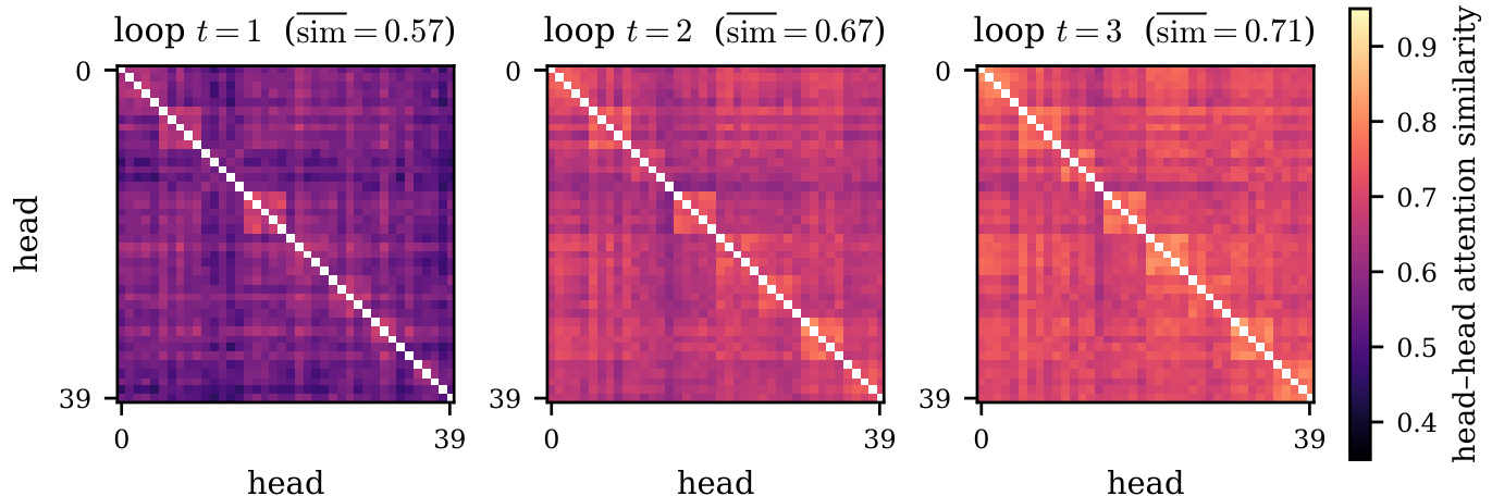
Figure 4. Head×head cosine similarity of the per-head attention distributions at loops $r = 1 , 2 , 3$ $\mathrm { P L T } _ { 3 } .$ , 500 held-out samples; self-similarity on the diagonal masked). Brighter cells indicate more redundant heads; sim is the mean off-diagonal similarity. Heads grow progressively more redundant across loops.
图 4. PLT3 在循环 $r = 1 , 2 , 3$ 中每头注意力分布的头间余弦相似度 (基于500个留出样本;对角线上的自相似度已遮蔽)。更亮的单元格表示头 (head) 之间冗余度更高;sim 为对角线外的平均相似度。随着循环推进,头的冗余程度逐渐加剧。
5. Discussion
5. 讨论
The per-loop analysis in section 4 reveals a consistent pattern: loop contributions are not uniform, and the interaction between representational gains and the cost imposed by the CLP offset shifts across loop index in a way that explains the non-monotonic performance curve.
第 4 节中的逐循环分析揭示了一个一致的模式:循环贡献并不均匀,表征增益与 CLP 偏移 (CLP offset) 带来的代价之间的交互作用会随循环索引变化,从而解释了非单调的性能曲线。
Loop 2 is the principal site of productive refinement. The second loop is the primary site of productive refinement: among the refinement loops it introduces the most coherent hidden-state update, the highest inter-loop attention divergence, and the greatest output-distribution shift, and it is where effective rank peaks. The first loop establishes the global KV cache used by all subsequent loops, so the quality of the loop-1 representations sets a ceiling on the information available to every later loop via the frozen global attention branch. The second loop then refines these representations using both fresh local context and the global cache, producing the largest net improvement.
Loop 2 是生产性精炼的主要场所。第二个循环是生产性精炼的核心环节:在所有精炼循环中,它引入了最连贯的隐藏状态更新,最高的循环间注意力差异,以及最大的输出分布偏移,并且有效秩在此达到峰值。第一个循环建立了供所有后续循环使用的全局 KV 缓存,因此循环 1 的表示质量为每个后续循环通过冻结的全局注意力分支能获取的信息设定了上限。随后,第二个循环利用全新的局部上下文和全局缓存对这些表示进行精炼,从而实现了最大的净改进。
Beyond loop 2: diminishing gains against a fixed cost. Beyond loop 2, the model faces compounding constraints. The effective rank declines from its loop-2 peak (representations become less diverse), so the shared block operates on a progressively lower-dimensional input, reducing the capacity for new computation. Meanwhile, the hidden-state update becomes oscillator y rather than convergent. At the same time, the intrinsic offset cost $\Omega ^ { ( r ) }$ remains roughly constant across loops: the CLP shift injects a comparable positional mismatch at every
超越循环2:固定成本下的收益递减。超越循环2,模型面临复合约束。有效秩 (effective rank) 从其在循环2的峰值下降 (表征变得不那么多样),因此共享块在逐渐降低维度的输入上运行,降低了新计算的能力。同时,隐藏状态更新变得振荡而非收敛。与此同时,固有偏移代价 $\Omega ^ { ( r ) }$ 在各循环间大致保持不变:CLP位移 (CLP shift) 在每一个

boundary. Because per-loop gains shrink rapidly while this offset cost stays fixed, the mismatch claims an ever-larger share of each loop’s net effect, so that beyond the second loop the cost increasingly outweighs the benefit.
在边界条件下,由于单次循环增益急剧衰减而该偏移成本保持不变,不匹配效应在每次循环净收益中所占比例持续扩大,导致其从第二轮循环后成本便逐步超过收益。
Practical guidelines for loop-count selection. These findings suggest several practical guidelines. The performance-saturation point identified in the analysis corresponds to a natural operating threshold for PLT deployment: $R = 2$ captures the dominant refinement step while incurring only a single additional forward pass. For finer-grained loop-count selection, the effective-rank trajectory is a lightweight per-model diagnostic that requires no exhaustive sweep: if effective rank is still rising at the candidate loop (representational diversity is not yet saturated), an additional loop may yield genuine refinement, whereas a rank that has begun to fall signals the onset of narrowing, after which further loops mostly add the fixed CLP offset cost without compensating gain.
循环计数选择的实用指南。这些发现揭示了若干实用指导原则。分析中确定的性能饱和点对应于 PLT 部署的自然运行阈值: $R = 2$ 捕获了主导的细化步骤,同时仅增加一次额外的正向传递。对于更精细的循环计数选择,有效秩轨迹是一种轻量级的逐模型诊断方法,无需进行穷举扫描:如果候选循环处的有效秩仍在上升 (表示表征多样性尚未饱和),则额外的循环可能产生真正的细化,而已开始下降的秩则标志着窄化出现的信号,在此之后进一步的循环主要增加固定的 CLP 偏移成本,而没有补偿性增益。
6. Related Work
6. 相关工作
6.1. Foundations of Looped Transformers
6.1. 循环Transformer (Looped Transformers) 的基础
The Universal Transformer (UT) [5] serves as the canonical starting point for looped LLM research. UT shares a single transformer block across depth and augments it with per-position adaptive computation time (ACT), a dynamic halting mechanism that allows individual tokens to exit the loop at different depths. Under certain conditions UT is provably Turing-complete, a theoretical property not generally attributable to fixed-depth transformers. The programmablecomputer interpretation of looped transformers was made precise by Giannou et al. [9], who demonstrated that a constant number of encoder layers in a loop suffices to emulate a generalpurpose instruction-set computer, including in-context learning via back-propagation. Yang et al. [18] further established that looped transformers match standard transformers on in-context learning benchmarks while using fewer than $1 0 %$ of the parameters, affirming their practical viability.
Universal Transformer (UT) [5] 是循环式大语言模型 (looped LLM) 研究的典范起点。UT 在深度上共享同一个 Transformer 块,并针对每个位置增加了自适应计算时间 (adaptive computation time, ACT),这是一种动态停止机制,允许各个 Token 在不同深度退出循环。在一定条件下,UT 可证明具有图灵完备性 (Turing-complete),这一理论性质通常不属于固定深度 Transformer。Giannou 等人 [9] 精确阐释了循环 Transformer 的可编程计算机 (programmable computer) 解释,证明循环中恒定数量的编码器层足以模拟通用指令集计算机,包括通过反向传播实现的上下文学习 (in-context learning)。Yang 等人 [18] 进一步证实,循环 Transformer 在上下文学习基准上与标准 Transformer 表现相当,同时参数使用量不到 $1 0 %$ ,确认了其实际可行性。

6.2. Test-Time Compute Scaling via Depth Recurrence
6.2. 通过深度递归实现测试时计算扩展 (Test-Time Compute Scaling via Depth Recurrence)
A central motivation for recent work on looped LLMs is test-time compute scaling: rather than generating additional tokens (as in chain-of-thought reasoning), a model can be run for more loops on harder inputs, performing implicit multi-step reasoning in latent space. Geiping et al. [8] demonstrated this at scale with Huginn-3.5B, a depth-recurrent transformer pretrained on 800B tokens that improves on reasoning benchmarks by applying up to 50 loops at inference, achieving an effective compute budget equivalent to a 50B-parameter model. Notably, this approach requires no specialized training data and can operate within smaller context windows than chain-of-thought methods. This latent reasoning paradigm, however, imposes a direct cost: each additional loop constitutes a full forward pass through the shared block, multiplying sequential inference latency by loopcount. More critically, standard KV-cache implementations store keys and values per layer per loop, causing memory to grow as $O ( l o o p c o u n t \cdot L )$ for a block of $L$ layers, a factor of loopcount overhead relative to the single-pass footprint. With too many loopcount, this overhead renders many architectures impractical for on-device or memory-constrained deployment. [15].
近期关于循环大语言模型 (Looped LLMs) 研究的一个核心动机是测试时计算扩展 (test-time compute scaling):模型无需生成额外 Token (如思维链推理方法),而是通过在更难输入上运行更多循环,在潜在空间中执行隐式多步推理。Geiping 等人 [8] 使用 Huginn-3.5B 模型进行了大规模验证——这是一个深度循环 Transformer,在 800B Token 上预训练,推理时最多应用 50 次循环即可提升推理基准表现,其有效计算预算相当于一个 500 亿参数模型的水平。值得注意的是,该方法无需专门训练数据,且能在比思维链方法更小的上下文窗口中运行。
然而,这种潜在推理范式带来了直接代价:每次额外循环都构成一次通过共享模块的完整前向传播,使得顺序推理延迟随循环次数成倍增长。更关键的是,标准 KV-cache 实现会为每个层每次循环存储键值对,导致对于包含 $L$ 层的模块,内存增长为 $O ( l o o p c o u n t \cdot L )$ ,这将产生相对于单次推理内存占用的循环次数倍开销。当循环次数过多时,这种开销会使许多架构难以在端侧或内存受限环境中部署 [15]。
6.3. Memory and Latency Reduction Techniques
6.3. 内存与延迟减少技术
Several works aim to retain the benefits of deep looping while reducing its inference cost. MELT decouples recurrence depth from memory by maintaining a single shared KV cache per layer across loops, updated through a learnable gating mechanism [15]. PLT instead targets latency by breaking sequential inter-loop dependencies with Cross-Loop Parallelism (CLP), and combines this with Gated Sliding-Window Attention (G-SWA) over shared global KV states and local current-loop context to keep memory nearly constant [16]. LT2 further reduces the cost of looped inference by replacing quadratic softmax attention with linear or sparse attention variants, leveraging recurrence for iterative memory refinement [6]. These methods improve the efficiency of looped computation, while our work focuses on the complementary question of how such efficiency mechanisms, especially PLT’s CLP offset, affect the usefulness of additional loops.
一些工作旨在保留深度循环的优势,同时降低其推理成本。MELT通过在各循环间维持每层单个共享KV缓存 (KV cache),并通过可学习的门控机制进行更新,从而将递归深度与内存解耦 [15]。PLT则通过跨循环并行 (Cross-Loop Parallelism, CLP) 打破顺序的循环间依赖来降低延迟,并将其与共享全局KV状态和局部当前循环上下文上的门控滑动窗口注意力 (Gated Sliding-Window Attention, G-SWA) 相结合,使内存几乎保持不变 [16]。LT2通过用线性或稀疏注意力变体替代二次softmax注意力,利用循环进行迭代记忆精炼,进一步降低了循环推理的成本 [6]。这些方法提高了循环计算的效率,而我们的工作则关注一个互补的问题:这类效率机制,尤其是PLT的CLP偏移,如何影响额外循环的有用性。

6.4. Architectural Variants
6.4. 架构变体
图 6.9 中的 Transformer 架构描述可能显得有些过于灵活,我们将它绘制出来的方式表明,仅解码器架构 (decoder-only architecture) 不需要编码器-解码器注意力 (encoder-decoder attention)。类似地,仅编码器架构 (encoder-only architecture) 无需任何形式的交叉注意力 (cross-attention)。图 6.9 中的原始设计思想确实表现为一种编码器-解码器架构 (encoder-decoder architecture),这在很多初始应用场景中很有意义。然而在实践中,过去几年中其他变体也发展起来,得到了广泛使用。这些架构变体的概述见图 6.13。
Figure 6.13: 流行的 Transformer 架构变体:仅编码器 (A),仅解码器 (B),以及编码器-解码器 (C)。在这类图示中,通常将输入放在底部,输出放在顶部,这意味着数据流自下而上。在仅解码器架构中,输出通常由输入序列经过偏移得到。
Beyond efficiency-oriented designs, another line of work explores richer looped architectures. Some methods relax strict weight sharing by adding lightweight loop-specific adaptation, such as depth-wise LoRA adapters for converting pretrained LLMs into recursive transformers [1]. Others restructure the recurrent computation itself, including Hyperloop Transformers with begin-middle-end partitioning and hyper-connections for inter-loop mixing [20], CART with a context-anchored recurrent core that cross-attends to frozen pre computed context tensors [2], and HRM-LM with fast and slow modules operating at different loop timescales [10]. Additional variants increase capacity or stability through mixture-of-experts feed forward layers [4], fixedpoint refinement with attractor modules [7], or post-training conversion of standard LLMs into looped encoder-reasoner-decoder architectures [13]. These works broaden the design space of looped Transformers, whereas our focus is complementary: we study how loop count affects the behavior of an efficient PLT architecture and why its performance saturates.
除了以效率为导向的设计之外,另一类研究探索了更丰富的循环架构 (looped architectures)。一些方法通过添加轻量级的循环特定适配来放松严格的权重共享,例如使用深度LoRA适配器将预训练大语言模型转换为递归Transformer [1]。另一些方法重构了循环计算本身,包括采用首-中-尾分区和用于跨循环混合的超连接 (hyper-connections) 的 Hyperloop Transformer [20],具有上下文锚定循环核心并交叉关注冻结预计算上下文张量的 CART [2],以及拥有以不同循环时间尺度运行的快慢模块的 HRM-LM [10]。其他变体通过混合专家前馈层 [4]、带有吸引子模块 (attractor modules) 的不动点精炼 [7],或将标准大语言模型训练后转换为循环编码器-推理器-解码器架构 [13],来提升容量或稳定性。这些工作拓宽了循环 Transformer 的设计空间,而我们的关注点与之互补:我们研究循环计数 (loop count) 如何影响高效 PLT 架构的行为,以及其性能为何会饱和。
6.5. Scaling Laws and Representation Dynamics
6.5. 规模法则与表征动态
Recent work has begun to study how looped models scale and how their internal representations evolve with recurrence depth. Scaling-law analyses show that increasing loop count yields diminishing returns: Schwethelm et al. [14] estimate that looping a block $r$ times is worth only $r ^ { 0 . 4 6 }$ unique parameters in validation loss, far below full equivalence to adding new layers. Complementary studies examine recurrent representation dynamics, finding that loop updates can become smaller, more orthogonal, or structured across multiple timescales [12]. Other work highlights stability as a central limitation: Yang et al. [19] show that performance can peak at an intermediate loop depth and then collapse, and propose fixed-point regular iz ation to stabilize recurrent computation. On the interpret ability side, prior analyses probe whether deeper recurrence corresponds to meaningful latent reasoning or natural-language-like intermediate computation, often finding mixed evidence and signs of representational degradation [3, 11]. Our work is closest in spirit to these representation-dynamics studies, but focuses specifically on PLT: we analyze how its efficiency mechanism changes the gain–cost profile across loops and why saturation occurs at a low loop count.
近期工作开始研究循环模型如何缩放,以及其内部表征如何随递归深度演化。缩放律分析表明,增加循环次数带来的收益递减:Schwethelm 等人 [14] 估计,将一个模块循环 $r$ 次,在验证损失上仅相当于 $r ^ { 0 . 4 6 }$ 个独立参数的效果,远不能等同于添加新的层。补充性研究考察了递归表征的动态变化,发现循环更新可能变得更小、更正交,或在多个时间尺度上呈现结构化 [12]。其他工作强调稳定性是核心限制因素:Yang 等人 [19] 表明,性能可能在某个中间循环深度达到峰值然后崩溃,并提出不动点正则化来稳定递归计算。在可解释性方面,已有分析探讨更深的递归是否对应有意义的潜在推理或类似自然语言的中间计算,但往往发现混杂的证据和表征退化的迹象 [3, 11]。我们的工作与这些表征动态研究的精神最为接近,但特别关注 PLT (Progressive Layer Training):分析其效率机制如何改变各循环中的增益-成本曲线,以及为何在较低的循环次数时出现饱和。
7. Conclusion
7. 结论
Looped Transformers provide an appealing mechanism for scaling latent computation without increasing parameter count, but their behavior under increasing loop count remains poorly understood. In this work, we study this problem in PLT through a gain–cost perspective: each additional loop may provide useful refinement, but the CLP offset also introduces a structural positional mismatch at every loop boundary. Our controlled loop-wise analysis shows that the second loop is the primary source of productive refinement, producing meaningful changes in hidden states, attention routing, and output distributions, while later loops yield diminishing and increasingly oscillator y updates. Because the CLP-induced mismatch remains approximately constant as marginal loop gains shrink, additional loops eventually become unproductive, explaining why PLT saturates at a small loop count. These findings provide interpret ability-grounded diagnostics for loop-count selection without exhaustive benchmark sweeps, and suggest future directions such as adaptive offset mechanisms, dynamic loop allocation, and a deeper understanding of how latent recurrence interacts with explicit chain-ofthought reasoning.
循环Transformer (Looped Transformers) 通过不增加参数量的方式扩展潜在计算,提供了一种极具吸引力的机制。然而,当循环次数增加时,其行为特性仍缺乏清晰理解。本研究从增益-成本视角切入,探讨PLT (Progressive Loop Transformer) 中的这一问题:每次额外循环可能提供有益优化,但CLP (Continuous Learned Positional) 偏移也会在每个循环边界引入结构性位置错配。我们的受控逐循环分析表明,第二个循环是产生有效优化的主要来源,能在隐藏状态、注意力路由和输出分布层面带来显著变化,而后续循环则呈现收益递减且振荡加剧的更新特征。由于CLP引发的错配程度基本保持不变,而边际循环增益不断缩小,额外循环最终会失去效用,这解释了为何PLT在较小循环次数时即达到饱和。这些发现为循环次数的选择提供了基于可解释性的诊断依据,无需进行穷举式基准测试,并指出了未来的研究方向,例如自适应偏移机制、动态循环分配,以及更深入理解潜在循环如何与外显思维链推理相互作用。
A. Forward-Pass Pseudocode
A. 前向传播伪代码 (Forward-Pass Pseudocode)
Algorithm 1 gives the PLT forward pass ( $\mu = 6 4$ throughout).
算法 1 给出了 PLT 前向传播过程 ( $\mu = 6 4$ 整体不变 )。
Algorithm 1 PLT Forward Pass $( w = 6 4 )$
算法1 PLT前向传播 $( w = 6 4 )$
B. Model Architecture Configurations
B. 模型架构配置
Table 5. Base model configuration used across all experiments.
| Hyperparameter | Value |
| Layers L | 14 |
| Hidden size d | 5120 |
| Attention heads H | 40 |
| KV groups (GQA) | 8 |
| Head dimension | 128 |
| FFN intermediate size | 27,648 |
| Activation | SwiGLU |
| Normalization | RMSNorm (ε = 10-5) |
| Position embedding | RoPE (base 5 × 10⁵) |
| Attention | Flash Attention, no dropout |
| QK LayerNorm | no |
| Bias in linear layers | no |
| Precision | bf16 |
| Vocabulary size | 76,800 |
| Total parameters | ~7B |
| Training tokens | 18T |
| Window size w | 64 (fixed) |
| CLP offset | enabled |
| Loop counts R analyzed | 1, 2,3,4 |
表 5: 用于所有实验的基础模型配置。
| 超参数 | 值 |
|---|---|
| 层数 L | 14 |
| 隐藏层大小 d | 5120 |
| 注意力头数 H | 40 |
| KV分组 ( GQA ) | 8 |
| 头维度 | 128 |
| FFN中间层大小 | 27,648 |
| 激活函数 | SwiGLU |
| 归一化 | RMSNorm ( ε = 10-5 ) |
| 位置嵌入 | RoPE ( base 5 × 10⁵ ) |
| 注意力机制 | Flash Attention,无 dropout |
| QK层归一化 | 否 |
| 线性层中的偏置 | 否 |
| 精度 | bf16 |
| 词汇表大小 | 76,800 |
| 总参数量 | ~7B |
| 训练 Token 数 | 18T |
| 窗口大小 w | 64 ( 固定 ) |
| CLP偏置 | 启用 |
| 分析的循环次数 R | 1, 2, 3, 4 |
The per-loop interpret ability analysis (section 4) is conducted across all loop counts, $R \in$ ${ 1 , 2 , 3 , 4 }$ .
每轮循环的可解释性分析 (第4节) 在所有循环次数 $R \in$ ${ 1 , 2 , 3 , 4 }$ 下进行。
C. Pre training Code-Data Composition
C. 预训练代码-数据组成
The pre training corpus is balanced at a 1:1 text-to-code token ratio (subsection 3.1). Table 6 breaks down the code half by programming language: the ten largest languages by token share, with the remaining 93 languages aggregated into “Others”. Shares are computed over code tokens only.
预训练语料库以 1:1 的文本与代码 Token 比例进行平衡 (第3.1节) 。表 6 按编程语言细分了代码部分:Token 占比最大的十种语言,其余 93 种语言归入“其他”。占比仅基于代码 Token 计算。
Table 6. Composition of the code portion of the 18T-token pre training mixture, as token share of all code tokens. Top-10 languages shown individually; the remaining 93 languages are grouped.
| Language | Token share (%) |
| Java | 10.3 |
| Python | 10.1 |
| JavaScript | 9.4 |
| Markdown TypeScript | 8.7 8.3 |
| C | 5.2 |
| C++ | 5.0 |
| PHP | 4.7 |
| C# | 4.0 |
| HTML | 3.7 |
| Others (93 languages) | 30.5 |
表 6. 18T-token 预训练混合语料中代码部分的构成,按所有代码 Token 的 Token 占比。前10种语言单独列出;其余93种语言归为一组。
| 语言 | Token 占比 (%) |
|---|---|
| Java | 10.3 |
| Python | 10.1 |
| JavaScript | 9.4 |
| Markdown TypeScript | 8.7 8.3 |
| C | 5.2 |
| C++ | 5.0 |
| PHP | 4.7 |
| C# | 4.0 |
| HTML | 3.7 |
| 其他 (93 种语言) | 30.5 |