XLNet: Generalized Auto regressive Pre training for Language Understanding
XLNet: 语言理解的广义自回归预训练
Abstract
摘要
With the capability of modeling bidirectional contexts, denoising auto encoding based pre training like BERT achieves better performance than pre training approaches based on auto regressive language modeling. However, relying on corrupting the input with masks, BERT neglects dependency between the masked positions and suffers from a pretrain-finetune discrepancy. In light of these pros and cons, we propose XLNet, a generalized auto regressive pre training method that (1) enables learning bidirectional contexts by maximizing the expected likelihood over all permutations of the factorization order and (2) overcomes the limitations of BERT thanks to its auto regressive formulation. Furthermore, XLNet integrates ideas from Transformer-XL, the state-of-the-art auto regressive model, into pre training. Empirically, under comparable experiment settings, XLNet outperforms BERT on 20 tasks, often by a large margin, including question answering, natural language inference, sentiment analysis, and document ranking.1.
基于双向上下文建模的能力,采用去噪自编码预训练的BERT相比基于自回归语言建模的预训练方法表现更优。然而,由于依赖掩码破坏输入,BERT忽略了被掩码位置间的依赖关系,并存在预训练与微调之间的差异。鉴于这些优缺点,我们提出了XLNet——一种广义自回归预训练方法,它通过以下两点实现突破:(1) 通过最大化因式分解顺序所有排列的期望似然来学习双向上下文;(2) 凭借自回归公式克服了BERT的局限性。此外,XLNet将当前最先进的自回归模型Transformer-XL的核心思想融入预训练阶段。实验表明,在可比实验设置下,XLNet在20项任务上显著超越BERT,包括问答、自然语言推理、情感分析和文档排序等任务。1.
1 Introduction
1 引言
Unsupervised representation learning has been highly successful in the domain of natural language processing [7, 22, 27, 28, 10]. Typically, these methods first pretrain neural networks on large-scale unlabeled text corpora, and then finetune the models or representations on downstream tasks. Under this shared high-level idea, different unsupervised pre training objectives have been explored in literature. Among them, auto regressive (AR) language modeling and auto encoding (AE) have been the two most successful pre training objectives.
无监督表示学习在自然语言处理领域取得了巨大成功 [7, 22, 27, 28, 10]。这些方法通常先在大规模无标注文本语料库上预训练神经网络,然后在下游任务上微调模型或表示。在这一共同的高层理念下,文献中探索了多种无监督预训练目标,其中自回归 (AR) 语言建模和自编码 (AE) 成为最成功的两种预训练目标。
AR language modeling seeks to estimate the probability distribution of a text corpus with an auto regressive model [7, 27, 28]. Specifically, given a text sequence $\mathbf{x}=(x_{1},\cdots,x_{T})$ , AR language modeling factorizes the likelihood into a forward product $\begin{array}{r}{p(\mathbf{x})=\prod_{t=1}^{T}p(x_{t}\mid\mathbf{x}_{<t})}\end{array}$ or a backward one $\begin{array}{r}{p(\mathbf{x})=\prod_{t=T}^{1}p(x_{t}\mid\mathbf{x}_{>t})}\end{array}$ . A parametric model (e.g. a neural network) is trained to model each conditional distribution. Since an AR language model is only trained to encode a uni-directional context (either forward or backward), it is not effective at modeling deep bidirectional contexts. On the contrary, downstream language understanding tasks often require bidirectional context information. This results in a gap between AR language modeling and effective pre training.
自回归(AR)语言建模旨在通过自回归模型估计文本语料库的概率分布[7,27,28]。具体而言,给定文本序列$\mathbf{x}=(x_{1},\cdots,x_{T})$,自回归语言建模将似然分解为前向乘积$\begin{array}{r}{p(\mathbf{x})=\prod_{t=1}^{T}p(x_{t}\mid\mathbf{x}_{<t})}\end{array}$或后向乘积$\begin{array}{r}{p(\mathbf{x})=\prod_{t=T}^{1}p(x_{t}\mid\mathbf{x}_{>t})}\end{array}$。通过参数化模型(如神经网络)来建模每个条件分布。由于自回归语言模型仅训练编码单向上下文(前向或后向),因此无法有效建模深度双向上下文。而下游语言理解任务通常需要双向上下文信息,这导致自回归语言建模与有效预训练之间存在差距。
In comparison, AE based pre training does not perform explicit density estimation but instead aims to reconstruct the original data from corrupted input. A notable example is BERT [10], which has been the state-of-the-art pre training approach. Given the input token sequence, a certain portion of tokens are replaced by a special symbol [MASK], and the model is trained to recover the original tokens from the corrupted version. Since density estimation is not part of the objective, BERT is allowed to utilize bidirectional contexts for reconstruction. As an immediate benefit, this closes the aforementioned bidirectional information gap in AR language modeling, leading to improved performance. However, the artificial symbols like [MASK] used by BERT during pre training are absent from real data at finetuning time, resulting in a pretrain-finetune discrepancy. Moreover, since the predicted tokens are masked in the input, BERT is not able to model the joint probability using the product rule as in AR language modeling. In other words, BERT assumes the predicted tokens are independent of each other given the unmasked tokens, which is oversimplified as high-order, long-range dependency is prevalent in natural language [9].
相比之下,基于自编码器 (AE) 的预训练并不执行显式密度估计,而是旨在从损坏的输入中重建原始数据。一个典型例子是 BERT [10],它曾是最先进的预训练方法。给定输入 token 序列后,模型会将部分 token 替换为特殊符号 [MASK],并通过训练从损坏版本中恢复原始 token。由于目标不包含密度估计,BERT 可以利用双向上下文进行重建。这一设计直接弥补了自回归 (AR) 语言建模中存在的双向信息缺口,从而提升了性能。然而,BERT 预训练时使用的 [MASK] 等人工符号在微调阶段的真实数据中并不存在,导致预训练与微调之间存在差异。此外,由于被预测的 token 在输入中被掩码,BERT 无法像 AR 语言建模那样通过乘积规则建模联合概率。换言之,BERT 假设在给定未掩码 token 的情况下,被预测的 token 彼此独立,这一假设过于简化,因为自然语言中普遍存在高阶长程依赖 [9]。
Faced with the pros and cons of existing language pre training objectives, in this work, we propose XLNet, a generalized auto regressive method that leverages the best of both AR language modeling and AE while avoiding their limitations.
面对现有语言预训练目标的优缺点,本文提出XLNet,这是一种广义自回归方法,它结合了自回归语言建模(AR)和自编码(AE)的优势,同时避免了它们的局限性。
• Firstly, instead of using a fixed forward or backward factorization order as in conventional AR models, XLNet maximizes the expected log likelihood of a sequence w.r.t. all possible permutations of the factorization order. Thanks to the permutation operation, the context for each position can consist of tokens from both left and right. In expectation, each position learns to utilize contextual information from all positions, i.e., capturing bidirectional context. • Secondly, as a generalized AR language model, XLNet does not rely on data corruption. Hence, XLNet does not suffer from the pretrain-finetune discrepancy that BERT is subject to. Meanwhile, the auto regressive objective also provides a natural way to use the product rule for factorizing the joint probability of the predicted tokens, eliminating the independence assumption made in BERT.
• 首先,与传统自回归(AR)模型使用固定前向或后向因子化顺序不同,XLNet针对所有可能的因子化顺序排列来最大化序列的期望对数似然。得益于排列操作,每个位置的上下文可以同时包含左右两侧的token。在期望情况下,每个位置都能学会利用所有位置的上下文信息,即捕获双向上下文。
• 其次,作为广义自回归语言模型,XLNet不依赖数据破坏。因此XLNet不会像BERT那样遭受预训练与微调不一致的问题。同时,自回归目标还提供了使用乘积规则分解预测token联合概率的自然方式,消除了BERT中的独立性假设。
In addition to a novel pre training objective, XLNet improves architectural designs for pre training.
除了新颖的预训练目标外,XLNet还改进了预训练的架构设计。
• Inspired by the latest advancements in AR language modeling, XLNet integrates the segment recurrence mechanism and relative encoding scheme of Transformer-XL [9] into pre training, which empirically improves the performance especially for tasks involving a longer text sequence. • Naively applying a Transformer(-XL) architecture to permutation-based language modeling does not work because the factorization order is arbitrary and the target is ambiguous. As a solution, we propose to re parameter ize the Transformer(-XL) network to remove the ambiguity.
• 受到AR语言建模最新进展的启发,XLNet将Transformer-XL [9]的分段循环机制和相对位置编码方案整合到预训练中,实验表明这尤其能提升涉及较长文本序列的任务性能。
• 直接将Transformer(-XL)架构应用于基于排列的语言建模是无效的,因为分解顺序是任意的且目标不明确。为此,我们提出对Transformer(-XL)网络进行重新参数化以消除这种模糊性。
Empirically, under comparable experiment setting, XLNet consistently outperforms BERT [10] on a wide spectrum of problems including GLUE language understanding tasks, reading comprehension tasks like SQuAD and RACE, text classification tasks such as Yelp and IMDB, and the ClueWeb09-B document ranking task.
实验表明,在可比的实验设置下,XLNet在包括GLUE语言理解任务、SQuAD和RACE等阅读理解任务、Yelp和IMDB等文本分类任务,以及ClueWeb09-B文档排序任务在内的广泛问题上,始终优于BERT [10]。
Related Work The idea of permutation-based AR modeling has been explored in [32, 12], but there are several key differences. Firstly, previous models aim to improve density estimation by baking an “orderless” inductive bias into the model while XLNet is motivated by enabling AR language models to learn bidirectional contexts. Technically, to construct a valid target-aware prediction distribution, XLNet incorporates the target position into the hidden state via two-stream attention while previous permutation-based AR models relied on implicit position awareness inherent to their MLP architectures. Finally, for both orderless NADE and XLNet, we would like to emphasize that “orderless” does not mean that the input sequence can be randomly permuted but that the model allows for different factorization orders of the distribution.
相关工作
基于排列的自回归(AR)建模思想已在[32,12]中被探讨,但存在几个关键差异。首先,先前模型旨在通过将"无序"归纳偏置融入模型来改进密度估计,而XLNet的动机是使AR语言模型能够学习双向上下文。技术上,为构建有效的目标感知预测分布,XLNet通过双流注意力将目标位置纳入隐藏状态,而先前的基于排列的AR模型依赖其MLP架构固有的隐式位置感知。最后,对于无序NADE和XLNet,我们强调"无序"并非指输入序列可随机排列,而是指模型允许分布的不同分解顺序。
Another related idea is to perform auto regressive denoising in the context of text generation [11], which only considers a fixed order though.
另一个相关想法是在文本生成过程中进行自回归去噪 [11],尽管这种方法只考虑固定顺序。
2 Proposed Method
2 提出的方法
2.1 Background
2.1 背景
In this section, we first review and compare the conventional AR language modeling and BERT for language pre training. Given a text sequence $\mathbf{x}=[x_{1},\cdots,x_{T}]$ , AR language modeling performs pre training by maximizing the likelihood under the forward auto regressive factorization:
在本节中,我们首先回顾并比较传统的自回归(AR)语言建模和BERT用于语言预训练的方法。给定一个文本序列$\mathbf{x}=[x_{1},\cdots,x_{T}]$,自回归语言建模通过前向自回归分解下的似然最大化进行预训练:
$$
\operatorname*{max}{\theta}\log p_{\theta}(\mathbf{x})=\sum_{t=1}^{T}\log p_{\theta}(x_{t}\mid\mathbf{x}{<t})=\sum_{t=1}^{T}\log\frac{\exp\left(h_{\theta}(\mathbf{x}{1:t-1})^{\top}e(x_{t})\right)}{\sum_{x^{\prime}}\exp\left(h_{\theta}(\mathbf{x}_{1:t-1})^{\top}e(x^{\prime})\right)},
$$
where $h_{\theta}(\mathbf{x}_{1:t-1})$ is a context representation produced by neural models, such as RNNs or Transformers, and $e(x)$ denotes the embedding of $x$ . In comparison, BERT is based on denoising auto-encoding. Specifically, for a text sequence $\mathbf{x}$ , BERT first constructs a corrupted version $\hat{\bf x}$ by randomly setting a portion (e.g. $15%$ ) of tokens in $\mathbf{x}$ to a special symbol [MASK]. Let the masked tokens be $\bar{\bf x}$ . The training objective is to reconstruct $\bar{\bf x}$ from $\hat{\bf x}$ :
其中 $h_{\theta}(\mathbf{x}_{1:t-1})$ 是由神经网络模型(如RNN或Transformer)生成的上下文表示,$e(x)$ 表示 $x$ 的嵌入。相比之下,BERT基于去噪自编码。具体来说,对于文本序列 $\mathbf{x}$,BERT首先通过随机将 $\mathbf{x}$ 中的一部分(例如 $15%$)token设为特殊符号[MASK]来构建损坏版本 $\hat{\bf x}$。设被遮蔽的token为 $\bar{\bf x}$,训练目标是从 $\hat{\bf x}$ 重建 $\bar{\bf x}$:
$$
\operatorname*{max}{\theta}\log p_{\theta}(\bar{\mathbf{x}}\mid\hat{\mathbf{x}})\approx\sum_{t=1}^{T}m_{t}\log p_{\theta}(x_{t}\mid\hat{\mathbf{x}})=\sum_{t=1}^{T}m_{t}\log\frac{\exp\left(H_{\theta}(\hat{\mathbf{x}}){t}^{\top}e(x_{t})\right)}{\sum_{x^{\prime}}\exp\left(H_{\theta}(\hat{\mathbf{x}})_{t}^{\top}e(x^{\prime})\right)},
$$
where $m_{t}=1$ indicates $x_{t}$ is masked, and $H_{\theta}$ is a Transformer that maps a length $T$ text sequence $\mathbf{x}$ into a sequence of hidden vectors $H_{\boldsymbol\theta}({\bf x})=[H_{\boldsymbol\theta}({\bf x})_{1},H_{\boldsymbol\theta}({\bf x})_{2},\cdot\cdot\cdot~,\bar{H_{\boldsymbol\theta}}({\bf x})_{T}]$ . The pros and cons of the two pre training objectives are compared in the following aspects:
其中 $m_{t}=1$ 表示 $x_{t}$ 被掩码,$H_{\theta}$ 是一个将长度为 $T$ 的文本序列 $\mathbf{x}$ 映射为隐藏向量序列 $H_{\boldsymbol\theta}({\bf x})=[H_{\boldsymbol\theta}({\bf x})_{1},H_{\boldsymbol\theta}({\bf x})_{2},\cdot\cdot\cdot~,\bar{H_{\boldsymbol\theta}}({\bf x})_{T}]$ 的 Transformer。这两种预训练目标在以下方面的优缺点进行了比较:
• Independence Assumption: As emphasized by the $\approx$ sign in Eq. (2), BERT factorizes the joint conditional probability $p(\bar{\bf x}\mid\hat{\bf x})$ based on an independence assumption that all masked tokens $\bar{\bf x}$ are separately reconstructed. In comparison, the AR language modeling objective (1) factorizes $p_{\boldsymbol{\theta}}(\mathbf{x})$ using the product rule that holds universally without such an independence assumption. • Input noise: The input to BERT contains artificial symbols like [MASK] that never occur in downstream tasks, which creates a pretrain-finetune discrepancy. Replacing [MASK] with original tokens as in [10] does not solve the problem because original tokens can be only used with a small probability — otherwise Eq. (2) will be trivial to optimize. In comparison, AR language modeling does not rely on any input corruption and does not suffer from this issue. • Context dependency: The AR representation $h_{\theta}(\mathbf{x}{1:t-1})$ is only conditioned on the tokens up to position $t$ (i.e. tokens to the left), while the BERT representation $H_{\boldsymbol\theta}(\mathbf{x})_{t}$ has access to the contextual information on both sides. As a result, the BERT objective allows the model to be pretrained to better capture bidirectional context.
• 独立性假设:如公式(2)中的≈符号所示,BERT基于独立性假设将联合条件概率p(x̄|x̂)分解,即所有被掩码的token x̄都是独立重建的。相比之下,自回归(AR)语言建模目标(1)使用普遍成立的乘积法则分解pθ(x),无需此类独立性假设。
• 输入噪声:BERT的输入包含[MASK]等下游任务中从未出现的人工符号,导致预训练与微调之间存在差异。如[10]所述用原始token替换[MASK]并不能解决问题,因为原始token只能以很小的概率使用——否则公式(2)的优化将失去意义。而AR语言建模不依赖任何输入破坏机制,因此不存在此问题。
• 上下文依赖性:AR表征hθ(x1:t-1)仅取决于位置t之前的token(即左侧token),而BERT表征Hθ(x)t能获取双向上下文信息。因此BERT目标使模型能通过预训练更好地捕捉双向上下文。
2.2 Objective: Permutation Language Modeling
2.2 目标:排列语言建模
According to the comparison above, AR language modeling and BERT possess their unique advantages over the other. A natural question to ask is whether there exists a pre training objective that brings the advantages of both while avoiding their weaknesses.
根据上述对比,AR (自回归) 语言建模和 BERT 各有独特优势。一个自然的问题是:是否存在一种预训练目标,能同时兼顾两者的优势并规避其弱点?
Borrowing ideas from orderless NADE [32], we propose the permutation language modeling objective that not only retains the benefits of AR models but also allows models to capture bidirectional contexts. Specifically, for a sequence $\mathbf{x}$ of length $T$ , there are $T!$ different orders to perform a valid auto regressive factorization. Intuitively, if model parameters are shared across all factorization orders, in expectation, the model will learn to gather information from all positions on both sides.
借鉴无序NADE [32]的思想,我们提出了排列语言建模目标,该目标不仅保留了自回归(AR)模型优势,还能让模型捕获双向上下文。具体而言,对于长度为$T$的序列$\mathbf{x}$,存在$T!$种不同的有效自回归分解顺序。直观来看,若所有分解顺序共享模型参数,模型将有望学会从两侧所有位置收集信息。
To formalize the idea, let $\mathcal{Z}{T}$ be the set of all possible permutations of the length $T$ index sequence $[1,2,\ldots,T]$ . We use $z_{t}$ and $\mathbf{z}{<t}$ to denote the $t$ -th element and the first $t-1$ elements of a permutation $\mathbf{z}\in\mathcal{Z}_{T}$ . Then, our proposed permutation language modeling objective can be expressed as follows:
为了形式化这一概念,设 $\mathcal{Z}{T}$ 为长度 $T$ 的索引序列 $[1,2,\ldots,T]$ 的所有可能排列集合。用 $z_{t}$ 和 $\mathbf{z}{<t}$ 分别表示排列 $\mathbf{z}\in\mathcal{Z}_{T}$ 的第 $t$ 个元素和前 $t-1$ 个元素。于是,我们提出的排列语言建模目标可表述为:
$$
\operatorname*{max}{\theta}\quad\mathbb{E}{\mathbf{z}\sim\mathcal{Z}{T}}\left[\sum_{t=1}^{T}\log p_{\theta}(x_{z_{t}}\mid\mathbf{x_{z}}_{<t})\right].
$$
$$
\operatorname*{max}{\theta}\quad\mathbb{E}{\mathbf{z}\sim\mathcal{Z}{T}}\left[\sum_{t=1}^{T}\log p_{\theta}(x_{z_{t}}\mid\mathbf{x_{z}}_{<t})\right].
$$
Essentially, for a text sequence $\mathbf{x}$ , we sample a factorization order $\mathbf{z}$ at a time and decompose the likelihood $p_{\boldsymbol{\theta}}(\mathbf{x})$ according to factorization order. Since the same model parameter $\theta$ is shared across all factorization orders during training, in expectation, $x_{t}$ has seen every possible element $x_{i}\neq x_{t}$ in the sequence, hence being able to capture the bidirectional context. Moreover, as this objective fits into the AR framework, it naturally avoids the independence assumption and the pretrain-finetune discrepancy discussed in Section 2.1.
本质上,对于文本序列 $\mathbf{x}$,我们每次采样一个分解顺序 $\mathbf{z}$,并根据该顺序分解似然 $p_{\boldsymbol{\theta}}(\mathbf{x})$。由于训练期间所有分解顺序共享相同的模型参数 $\theta$,从期望上看,$x_{t}$ 已观测到序列中所有可能的元素 $x_{i}\neq x_{t}$,因此能够捕获双向上下文。此外,由于该目标符合自回归 (AR) 框架,自然避免了第2.1节讨论的独立性假设与预训练-微调差异问题。
Remark on Permutation The proposed objective only permutes the factorization order, not the sequence order. In other words, we keep the original sequence order, use the positional encodings corresponding to the original sequence, and rely on a proper attention mask in Transformers to achieve permutation of the factorization order. Note that this choice is necessary, since the model will only encounter text sequences with the natural order during finetuning.
关于排列的说明
提出的目标仅对分解顺序进行排列,而非序列顺序。换言之,我们保持原始序列顺序,使用与原始序列对应的位置编码,并依靠Transformer中的适当注意力掩码来实现分解顺序的排列。需要注意的是,这一选择是必要的,因为在微调阶段模型只会遇到具有自然顺序的文本序列。
To provide an overall picture, we show an example of predicting the token $x_{3}$ given the same input sequence $\mathbf{x}$ but under different factorization orders in the Appendix A.7 with Figure 4.
为了提供整体概览,我们在附录A.7的图4中展示了给定相同输入序列$\mathbf{x}$但采用不同分解顺序时预测token$x_{3}$的示例。
2.3 Architecture: Two-Stream Self-Attention for Target-Aware Representations
2.3 架构:面向目标感知表征的双流自注意力机制
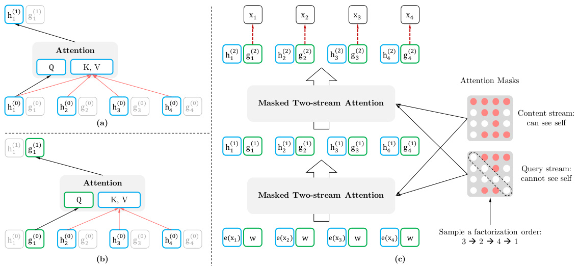
Figure 1: (a): Content stream attention, which is the same as the standard self-attention. (b): Query stream attention, which does not have access information about the content $x_{z_{t}}$ . (c): Overview of the permutation language modeling training with two-stream attention.
图 1: (a) 内容流注意力机制,与标准自注意力机制相同。(b) 查询流注意力机制,无法获取内容 $x_{z_{t}}$ 的相关信息。(c) 采用双流注意力机制的排列语言模型训练概览。
While the permutation language modeling objective has desired properties, naive implementation with standard Transformer parameter iz ation may not work. To see the problem, assume we parameter ize the next-token distribution $p_{\theta}(X_{z_{t}}\mid\mathbf{x}{\mathbf{z}{<t}})$ using the standard Softmax formulation, i.e., $p_{\theta}(X_{z_{t}}=$ $\begin{array}{r}{x\mid\mathbf{x_{z}}{<t}\big)=\frac{\exp\left(e(x)^{\top}h_{\theta}(\mathbf{x_{z}}{<t})\right)}{\sum_{x^{\prime}}\exp\left(e(x^{\prime})^{\top}h_{\theta}(\mathbf{x_{z}}{<t})\right)}}\end{array}$ Pxe′x epx(pe((ex()x′)hθ⊤(hxθz(<xtz)<)t)) , where hθ(xz<t) denotes the hidden representation of xz<t produced by the shared Transformer network after proper masking. Now notice that the representation $\bar{h}{\theta}(\mathbf{x}{\mathbf{z}{<t}})$ does not depend on which position it will predict, i.e., the value of $z_{t}$ . Consequently, the same distribution is predicted regardless of the target position, which is not able to learn useful representations (see Appendix A.1 for a concrete example). To avoid this problem, we propose to re-parameter ize the next-token distribution to be target position aware:
虽然排列语言建模目标具有理想特性,但使用标准Transformer参数化的朴素实现可能无法奏效。为说明问题,假设我们采用标准Softmax公式参数化下一个token分布$p_{\theta}(X_{z_{t}}\mid\mathbf{x}{\mathbf{z}{<t}})$,即$p_{\theta}(X_{z_{t}}=$$\begin{array}{r}{x\mid\mathbf{x_{z}}{<t}\big)=\frac{\exp\left(e(x)^{\top}h_{\theta}(\mathbf{x_{z}}{<t}\right)}{\sum_{x^{\prime}}\exp\left(e(x^{\prime})^{\top}h_{\theta}(\mathbf{x_{z}}{<t}\right)}}\end{array}$Pxe′x epx(pe((ex()x′)hθ⊤(hxθz(<xtz)<)t)),其中hθ(xz<t)表示经过适当掩码处理后,共享Transformer网络生成的xz<t隐藏表示。需注意表示$\bar{h}{\theta}(\mathbf{x}{\mathbf{z}{<t}})$不依赖于其预测位置$z_{t}$,导致无论目标位置如何都会预测相同分布,从而无法学习有效表示(具体示例见附录A.1)。为避免此问题,我们提出重新参数化下一个token分布以感知目标位置:
$$
p_{\theta}(X_{z_{t}}=x\mid\mathbf{x}{z_{<t}})=\frac{\exp\left(e(x)^{\top}g_{\theta}(\mathbf{x}{\mathbf{z}{<t}},z_{t})\right)}{\sum_{x^{\prime}}\exp\left(e(x^{\prime})^{\top}g_{\theta}(\mathbf{x}{\mathbf{z}{<t}},z_{t})\right)},
$$
$$
p_{\theta}(X_{z_{t}}=x\mid\mathbf{x}{z_{<t}})=\frac{\exp\left(e(x)^{\top}g_{\theta}(\mathbf{x}{\mathbf{z}{<t}},z_{t})\right)}{\sum_{x^{\prime}}\exp\left(e(x^{\prime})^{\top}g_{\theta}(\mathbf{x}{\mathbf{z}{<t}},z_{t})\right)},
$$
where $g_{\theta}\big(\mathbf{x_{z}}{<t},z_{t}\big)$ denotes a new type of representations which additionally take the target position $z_{t}$ as input.
其中 $g_{\theta}\big(\mathbf{x_{z}}{<t},z_{t}\big)$ 表示一种新型表征方式,该表征额外将目标位置 $z_{t}$ 作为输入。
Two-Stream Self-Attention While the idea of target-aware representations removes the ambiguity in target prediction, how to formulate $g_{\theta}\left(\mathbf{x_{z}}{<t},z_{t}\right)$ remains a non-trivial problem. Among other possibilities, we propose to “stand” at the target position $z_{t}$ and rely on the position $z_{t}$ to gather information from the context $\mathbf{x_{z}}{<t}$ through attention. For this parameter iz ation to work, there are two requirements that are contradictory in a standard Transformer architecture: (1) to predict the token $x_{z_{t}}$ , $g_{\theta}(\mathbf{x_{z}}{<t},z_{t})$ should only use the position $z_{t}$ and not the content $x_{z_{t}}$ , otherwise the objective becomes trivial; (2) to predict the other tokens $x_{z_{j}}$ with $j>t$ , $g_{\theta}\big(\mathbf{x_{z}}{<t},z_{t}\big)$ should also encode the content $x_{z_{t}}$ to provide full contextual information. To resolve such a contradiction, we propose to use two sets of hidden representations instead of one:
双流自注意力机制
虽然目标感知表示的概念消除了目标预测中的歧义,但如何构建 $g_{\theta}\left(\mathbf{x_{z}}{<t},z_{t}\right)$ 仍是一个关键问题。我们提出一种方案:以目标位置 $z_{t}$ 为观测点,通过注意力机制从上下文 $\mathbf{x_{z}}{<t}$ 中聚合信息。这种参数化方式在标准Transformer架构中面临两个相互矛盾的要求:(1) 预测Token $x_{z_{t}}$ 时,$g_{\theta}(\mathbf{x_{z}}{<t},z_{t})$ 应仅使用位置 $z_{t}$ 而忽略内容 $x_{z_{t}}$,否则目标函数将失效;(2) 预测后续Token $x_{z_{j}}$ (其中 $j>t$) 时,$g_{\theta}\big(\mathbf{x_{z}}{<t},z_{t}\big)$ 需编码内容 $x_{z_{t}}$ 以提供完整上下文信息。为解决这一矛盾,我们提出采用两组隐藏表示而非单一表示:
• The content representation $h_{\theta}(\mathbf{x}{\mathbf{z}{\le t}})$ , or abbreviated as $h_{z_{t}}$ , which serves a similar role to the standard hidden states in Transformer. This representation encodes both the context and $x_{z_{t}}$ itself. • The query representation $g_{\theta}\left(\mathbf{x_{z}}{<t},z_{t}\right)$ , or abbreviated as $g_{z_{t}}$ , which only has access to the contextual information $\mathbf{x_{z}}{<t}$ and the position $z_{t}$ , but not the content $x_{z_{t}}$ , as discussed above.
• 内容表示 $h_{\theta}(\mathbf{x}{\mathbf{z}{\le t}})$ (简写为 $h_{z_{t}}$),其作用类似于Transformer中的标准隐藏状态。该表示同时编码了上下文信息和 $x_{z_{t}}$ 本身。
• 查询表示 $g_{\theta}\left(\mathbf{x_{z}}{<t},z_{t}\right)$ (简写为 $g_{z_{t}}$),仅能访问上下文信息 $\mathbf{x_{z}}{<t}$ 和位置 $z_{t}$,但无法获取内容 $x_{z_{t}}$,如上文所述。
Computationally, the first layer query stream is initialized with a trainable vector, i.e. $g_{i}^{(0)}=w$ , while the content stream is set to the corresponding word embedding, i.e. $h_{i}^{(0)}=e(x_{i})$ . For each self-attention layer $m=1,\ldots,M$ , the two streams of representations are schematically 2 updated with a shared set of parameters as follows (illustrated in Figures 1 (a) and (b)):
在计算上,第一层查询流 (query stream) 初始化为可训练向量,即 $g_{i}^{(0)}=w$,而内容流 (content stream) 设置为对应的词嵌入 (word embedding),即 $h_{i}^{(0)}=e(x_{i})$。对于每个自注意力层 $m=1,\ldots,M$,这两个表示流通过共享参数集按以下方式更新(如图 1(a) 和 (b) 所示):
$$
\begin{array}{r l}&{g_{z_{t}}^{(m)}\gets\mathrm{Attention}(\mathsf{Q}=g_{z_{t}}^{(m-1)},\mathbf{KV}=\mathbf{h}_{z<t}^{(m-1)};\theta),\quad(\mathrm{query~stream};\mathrm{~use~}z_{t}\mathrm{~but~cannot~see~}x_{z_{t}})}\ &{h_{z_{t}}^{(m)}\gets\mathrm{Attention}(\mathsf{Q}=h_{z_{t}}^{(m-1)},\mathbf{KV}=\mathbf{h}_{z<t}^{(m-1)};\theta),\quad(\mathrm{content~stream};\mathrm{~use~both~}z_{t}\mathrm{~and~}x_{z_{t}}).}\end{array}
$$
$$
\begin{array}{r l}&{g_{z_{t}}^{(m)}\gets\mathrm{Attention}(\mathsf{Q}=g_{z_{t}}^{(m-1)},\mathbf{KV}=\mathbf{h}_{z<t}^{(m-1)};\theta),\quad(\mathrm{query~stream};\mathrm{~use~}z_{t}\mathrm{~but~cannot~see~}x_{z_{t}})}\ &{h_{z_{t}}^{(m)}\gets\mathrm{Attention}(\mathsf{Q}=h_{z_{t}}^{(m-1)},\mathbf{KV}=\mathbf{h}_{z<t}^{(m-1)};\theta),\quad(\mathrm{content~stream};\mathrm{~use~both~}z_{t}\mathrm{~and~}x_{z_{t}}).}\end{array}
$$
where Q, K, V denote the query, key, and value in an attention operation [33]. The update rule of the content representations is exactly the same as the standard self-attention, so during finetuning, we can simply drop the query stream and use the content stream as a normal Transformer(-XL). Finally, we can use the last-layer query representation gzt $g_{z_{t}}^{(M)}$ to compute Eq. (4).
其中 Q、K、V 表示注意力操作中的查询 (query)、键 (key) 和值 (value) [33]。内容表征的更新规则与标准自注意力完全相同,因此在微调时,我们可以直接丢弃查询流并将内容流作为常规 Transformer(-XL) 使用。最终,我们可以使用最后一层的查询表征 gzt $g_{z_{t}}^{(M)}$ 来计算公式 (4)。
Partial Prediction While the permutation language modeling objective (3) has several benefits, it is a much more challenging optimization problem due to the permutation and causes slow convergence in preliminary experiments. To reduce the optimization difficulty, we choose to only predict the last tokens in a factorization order. Formally, we split $\mathbf{z}$ into a non-target sub sequence $\mathbf{z}{\leq c}$ and a target sub sequence $\mathbf{z}_{>c}$ , where $c$ is the cutting point. The objective is to maximize the log-likelihood of the target sub sequence conditioned on the non-target sub sequence, i.e.,
部分预测
虽然排列语言建模目标 (3) 具有多个优势,但由于排列的存在,它成为一个更具挑战性的优化问题,并在初步实验中导致收敛速度较慢。为了降低优化难度,我们选择仅预测分解顺序中的最后几个 token。形式上,我们将 $\mathbf{z}$ 划分为非目标子序列 $\mathbf{z}{\leq c}$ 和目标子序列 $\mathbf{z}_{>c}$ ,其中 $c$ 为切割点。目标是在给定非目标子序列的条件下,最大化目标子序列的对数似然,即
$$
\operatorname*{max}{\theta}\quad\mathbb{E}{\mathbf{z}\sim\mathcal{Z}{T}}\left[\log p_{\theta}(\mathbf{x}{\mathbf{z}{>c}}\mid\mathbf{x}{\mathbf{z}{\leq c}})\right]=\mathbb{E}{\mathbf{z}\sim\mathcal{Z}{T}}\left[\sum_{t=c+1}^{|\mathbf{z}|}\log p_{\theta}(x_{z_{t}}\mid\mathbf{x}{\mathbf{z}_{<t}})\right].
$$
$$
\operatorname*{max}{\theta}\quad\mathbb{E}{\mathbf{z}\sim\mathcal{Z}{T}}\left[\log p_{\theta}(\mathbf{x}{\mathbf{z}{>c}}\mid\mathbf{x}{\mathbf{z}{\leq c}})\right]=\mathbb{E}{\mathbf{z}\sim\mathcal{Z}{T}}\left[\sum_{t=c+1}^{|\mathbf{z}|}\log p_{\theta}(x_{z_{t}}\mid\mathbf{x}{\mathbf{z}_{<t}})\right].
$$
Note that $\mathbf{z}_{>c}$ is chosen as the target because it possesses the longest context in the sequence given the current factorization order $\mathbf{z}$ . A hyper parameter $K$ is used such that about $1/K$ tokens are selected for predictions; i.e., $\left|\mathbf{z}\right|/(\left|\mathbf{z}\right|-c)\overset{.}{\approx}\bar{K}$ . For unselected tokens, their query representations need not be computed, which saves speed and memory.
注意,选择 $\mathbf{z}_{>c}$ 作为目标是因为在给定当前分解顺序 $\mathbf{z}$ 的情况下,它在序列中拥有最长的上下文。使用超参数 $K$,使得大约 $1/K$ 的 token 被选中用于预测;即 $\left|\mathbf{z}\right|/(\left|\mathbf{z}\right|-c)\overset{.}{\approx}\bar{K}$。对于未被选中的 token,无需计算它们的查询表示,从而节省速度和内存。
2.4 Incorporating Ideas from Transformer-XL
2.4 融入Transformer-XL思想
Since our objective function fits in the AR framework, we incorporate the state-of-the-art AR language model, Transformer-XL [9], into our pre training framework, and name our method after it. We integrate two important techniques in Transformer-XL, namely the relative positional encoding scheme and the segment recurrence mechanism. We apply relative positional encodings based on the original sequence as discussed earlier, which is straightforward. Now we discuss how to integrate the recurrence mechanism into the proposed permutation setting and enable the model to reuse hidden states from previous segments. Without loss of generality, suppose we have two segments taken from a long sequence s; i.e., $\tilde{\mathbf{x}}=\mathbf{s}{1:T}$ and $\mathbf{x}=\mathbf{s}_{T+1:2T}$ . Let $\tilde{\mathbf{z}}$ and $\mathbf{z}$ be permutations of $[1\cdots T]$ and $[T+1\cdots2T]$ respectively. Then, based on the permutation $\tilde{\mathbf{z}}$ , we process the first segment, and then cache the obtained content representations $\tilde{\mathbf{h}}^{(m)}$ for each layer $m$ . Then, for the next segment $\mathbf{x}$ , the attention update with memory can be written as
由于我们的目标函数符合自回归(AR)框架,我们将最先进的自回归语言模型Transformer-XL[9]纳入预训练框架,并以其命名我们的方法。我们整合了Transformer-XL中的两项关键技术:相对位置编码方案和分段循环机制。基于前文讨论的原始序列,我们直接应用了相对位置编码。接下来讨论如何将循环机制融入提出的排列设置中,使模型能够复用前序分段的隐藏状态。不失一般性,假设从长序列s中提取两个分段:$\tilde{\mathbf{x}}=\mathbf{s}{1:T}$和$\mathbf{x}=\mathbf{s}_{T+1:2T}$。设$\tilde{\mathbf{z}}$和$\mathbf{z}$分别为$[1\cdots T]$和$[T+1\cdots2T]$的排列。基于排列$\tilde{\mathbf{z}}$处理第一分段后,缓存各层$m$获得的内容表示$\tilde{\mathbf{h}}^{(m)}$。对于后续分段$\mathbf{x}$,带记忆的注意力更新可表示为
$$
h_{z_{t}}^{(m)}\gets\mathrm{Attention}(\mathbf{Q}=h_{z_{t}}^{(m-1)},\mathbf{K}\mathbf{V}=\left[\tilde{\mathbf{h}}^{(m-1)},\mathbf{h}{\mathbf{z}_{\leq t}}^{(m-1)}\right];\theta)
$$
$$
h_{z_{t}}^{(m)}\gets\mathrm{Attention}(\mathbf{Q}=h_{z_{t}}^{(m-1)},\mathbf{K}\mathbf{V}=\left[\tilde{\mathbf{h}}^{(m-1)},\mathbf{h}{\mathbf{z}_{\leq t}}^{(m-1)}\right];\theta)
$$
where $[.,.]$ denotes concatenation along the sequence dimension. Notice that positional encodings only depend on the actual positions in the original sequence. Thus, the above attention update is independent of $\tilde{\mathbf{z}}$ once the representations $\tilde{\mathbf{h}}^{(m)}$ are obtained. This allows caching and reusing the memory without knowing the factorization order of the previous segment. In expectation, the model learns to utilize the memory over all factorization orders of the last segment. The query stream can be computed in the same way. Finally, Figure 1 (c) presents an overview of the proposed permutation language modeling with two-stream attention (see Appendix A.7 for more detailed illustration).
其中 $[.,.]$ 表示沿序列维度的拼接。请注意位置编码仅依赖于原始序列中的实际位置。因此,一旦获得表征 $\tilde{\mathbf{h}}^{(m)}$ ,上述注意力更新便与 $\tilde{\mathbf{z}}$ 无关。这使得我们无需知晓前一片段的分解顺序即可缓存并复用记忆。在期望情况下,模型会学习利用最后片段所有分解顺序的记忆。查询流的计算方式与之相同。最终,图1(c) 展示了采用双流注意力的排列语言建模方案概览 (更详细说明参见附录 A.7)。
2.5 Modeling Multiple Segments
2.5 多段建模
Many downstream tasks have multiple input segments, e.g., a question and a context paragraph in question answering. We now discuss how we pretrain XLNet to model multiple segments in the auto regressive framework. During the pre training phase, following BERT, we randomly sample two segments (either from the same context or not) and treat the concatenation of two segments as one sequence to perform permutation language modeling. We only reuse the memory that belongs to the same context. Specifically, the input to our model is the same as BERT: [CLS, A, SEP, B, SEP], where “SEP” and “CLS” are two special symbols and “A” and “B” are the two segments. Although we follow the two-segment data format, XLNet-Large does not use the objective of next sentence prediction [10] as it does not show consistent improvement in our ablation study (see Section 3.4).
许多下游任务包含多个输入片段,例如问答中的问题和上下文段落。下面我们将讨论XLNet如何在自回归框架中对多片段进行预训练。在预训练阶段,我们遵循BERT的做法,随机抽取两个片段(可能来自相同或不同上下文)并将它们拼接为一个序列进行排列语言建模。我们仅复用属于同一上下文的记忆。具体而言,模型输入格式与BERT相同:[CLS, A, SEP, B, SEP],其中"SEP"和"CLS"是特殊符号,"A"和"B"代表两个片段。尽管采用双片段数据格式,但XLNet-Large未使用下一句预测目标[10],因为消融研究(见第3.4节)显示该目标未能带来稳定提升。
Relative Segment Encodings Architecturally, different from BERT that adds an absolute segment embedding to the word embedding at each position, we extend the idea of relative encodings from Transformer-XL to also encode the segments. Given a pair of positions $i$ and $j$ in the sequence, if $i$ and $j$ are from the same segment, we use a segment encoding $\mathbf{s}{i j}=\mathbf{s}{+}$ or otherwise $\mathbf{s}{i j}=\mathbf{s}{-}$ , where $\mathbf{s}{+}$ and $\mathbf{s}{-}$ are learnable model parameters for each attention head. In other words, we only consider whether the two positions are within the same segment, as opposed to considering which specific segments they are from. This is consistent with the core idea of relative encodings; i.e., only modeling the relationships between positions. When $i$ attends to $j$ , the segment encoding $\mathbf{s}{i j}$ is used to compute an attention weight $a_{i j}=({\bf q}{i}+{\bf b})^{\top}{\bf s}{i j}$ , where $\mathbf{q}{i}$ is the query vector as in a standard attention operation and $\mathbf{b}$ is a learnable head-specific bias vector. Finally, the value $a_{i j}$ is added to the normal attention weight. There are two benefits of using relative segment encodings. First, the inductive bias of relative encodings improves generalization [9]. Second, it opens the possibility of finetuning on tasks that have more than two input segments, which is not possible using absolute segment encodings.
相对分段编码架构
与BERT在每个位置的词嵌入上添加绝对分段嵌入不同,我们扩展了Transformer-XL的相对编码思想,使其也能对分段进行编码。给定序列中的一对位置$i$和$j$,如果$i$和$j$来自同一分段,则使用分段编码$\mathbf{s}{i j}=\mathbf{s}{+}$,否则使用$\mathbf{s}{i j}=\mathbf{s}{-}$,其中$\mathbf{s}{+}$和$\mathbf{s}{-}$是每个注意力头可学习的模型参数。换句话说,我们只考虑两个位置是否在同一分段内,而不考虑它们来自哪个特定分段。这与相对编码的核心思想一致,即仅建模位置之间的关系。当$i$关注$j$时,分段编码$\mathbf{s}{i j}$用于计算注意力权重$a_{i j}=({\bf q}{i}+{\bf b})^{\top}{\bf s}{i j}$,其中$\mathbf{q}{i}$是标准注意力操作中的查询向量,$\mathbf{b}$是特定于注意力头的可学习偏置向量。最后,将值$a_{i j}$添加到常规注意力权重中。使用相对分段编码有两个好处:首先,相对编码的归纳偏置提高了泛化能力[9];其次,它为在具有两个以上输入分段的任务上进行微调提供了可能性,而绝对分段编码无法实现这一点。
2.6 Discussion
2.6 讨论
Comparing Eq. (2) and (5), we observe that both BERT and XLNet perform partial prediction, i.e., only predicting a subset of tokens in the sequence. This is a necessary choice for BERT because if all tokens are masked, it is impossible to make any meaningful predictions. In addition, for both BERT and XLNet, partial prediction plays a role of reducing optimization difficulty by only predicting tokens with sufficient context. However, the independence assumption discussed in Section 2.1 disables BERT to model dependency between targets.
比较式 (2) 和式 (5) 可以发现,BERT 和 XLNet 都采用了部分预测 (partial prediction) 策略,即仅预测序列中的部分 token。对于 BERT 而言这是必然选择,因为若全部 token 都被掩码,模型将无法进行有效预测。此外,部分预测对两者都具有降低优化难度的作用,只需基于充分上下文预测特定 token。但如第 2.1 节所述,独立性假设导致 BERT 无法建模预测目标间的依赖关系。
To better understand the difference, let’s consider a concrete example [New, York, is, a, city]. Suppose both BERT and XLNet select the two tokens [New, York] as the prediction targets and maximize $\log p(\mathrm{NewYork~}|$ is a city). Also suppose that XLNet samples the factorization order [is, a, city, New, York]. In this case, BERT and XLNet respectively reduce to the following objectives:
为了更好地理解差异,让我们看一个具体例子 [New, York, is, a, city]。假设 BERT 和 XLNet 都选择两个 token [New, York] 作为预测目标,并最大化 $\log p(\mathrm{NewYork~}|$ is a city)。再假设 XLNet 采样了因子分解顺序 [is, a, city, New, York]。此时 BERT 和 XLNet 分别简化为以下目标:
$$
{\mathcal{I}}_{\mathrm{XLNet}}=\log p({\mathrm{New~}}\vert{\mathrm{ is a city}})+\log p({\mathrm{York~}}\vert{\mathrm{New}},{\mathrm{is a~city}}).
$$
Notice that XLNet is able to capture the dependency between the pair (New, York), which is omitted by BERT. Although in this example, BERT learns some dependency pairs such as (New, city) and (York, city), it is obvious that XLNet always learns more dependency pairs given the same target and contains “denser” effective training signals.
注意到XLNet能够捕捉到(New, York)之间的依赖关系,而BERT忽略了这一点。尽管在这个例子中,BERT学习到了一些依赖对,如(New, city)和(York, city),但很明显,在给定相同目标的情况下,XLNet总是学习到更多的依赖对,并包含"更密集"的有效训练信号。
For more formal analysis and further discussion, please refer to Appendix A.5.
如需更正式的分析和进一步讨论,请参阅附录 A.5。
3 Experiments
3 实验
3.1 Pre training and Implementation
3.1 预训练与实现
Following BERT [10], we use the Books Corpus [40] and English Wikipedia as part of our pre training data, which have 13GB plain text combined. In addition, we include Giga5 (16GB text) [26], ClueWeb 2012-B (extended from [5]), and Common Crawl [6] for pre training. We use heuristics to aggressively filter out short or low-quality articles for ClueWeb 2012-B and Common Crawl, which results in 19GB and 110GB text respectively. After token iz ation with Sentence Piece [17], we obtain 2.78B, 1.09B, 4.75B, 4.30B, and 19.97B subword pieces for Wikipedia, Books Corpus, Giga5, ClueWeb, and Common Crawl respectively, which are 32.89B in total.
遵循BERT [10]的做法,我们使用Books Corpus [40]和英文维基百科作为预训练数据的一部分,两者合计包含13GB纯文本。此外,我们还加入了Giga5(16GB文本)[26]、ClueWeb 2012-B(基于[5]扩展)以及Common Crawl [6]进行预训练。针对ClueWeb 2012-B和Common Crawl,我们采用启发式方法严格过滤短文本或低质量文章,最终分别获得19GB和110GB文本。通过Sentence Piece [17]进行Token化处理后,维基百科、Books Corpus、Giga5、ClueWeb和Common Crawl分别生成2.78B、1.09B、4.75B、4.30B和19.97B子词片段,总计32.89B。
Our largest model XLNet-Large has the same architecture hyper parameters as BERT-Large, which results in a similar model size. During pre training, we always use a full sequence length of 512. Firstly, to provide a fair comparison with BERT (section 3.2), we also trained XLNet-Large-wikibooks on Books Corpus and Wikipedia only, where we reuse all pre training hyper-parameters as in the original BERT. Then, we scale up the training of XLNet-Large by using all the datasets described above. Specifically, we train on 512 TPU v3 chips for 500K steps with an Adam weight decay optimizer, linear learning rate decay, and a batch size of 8192, which takes about 5.5 days. It was observed that the model still underfits the data at the end of training. Finally, we perform ablation study (section 3.4) based on the XLNet-Base-wikibooks.
我们最大的模型XLNet-Large采用了与BERT-Large相同的架构超参数,因此模型规模相近。预训练阶段始终使用512的完整序列长度。首先,为与BERT进行公平对比(见3.2节),我们仅在Books Corpus和Wikipedia数据上训练XLNet-Large-wikibooks,并完全复用原始BERT的所有预训练超参数。随后,我们通过使用前述全部数据集来扩展XLNet-Large的训练规模。具体而言,我们在512块TPU v3芯片上进行了50万步训练,采用Adam权重衰减优化器、线性学习率衰减策略,批处理大小为8192,耗时约5.5天。观察发现模型在训练结束时仍存在欠拟合现象。最后,我们基于XLNet-Base-wikibooks进行了消融实验(见3.4节)。
Since the recurrence mechanism is introduced, we use a bidirectional data input pipeline where each of the forward and backward directions takes half of the batch size. For training XLNet-Large, we set the partial prediction constant $K$ as 6 (see Section 2.3). Our finetuning procedure follows BERT [10] except otherwise specified3. We employ an idea of span-based prediction, where we first sample a length $L\in[1,\cdots,5]$ , and then randomly select a consecutive span of $L$ tokens as prediction targets within a context of $(\Bar{K}L)$ tokens.
由于引入了递归机制,我们采用双向数据输入管道,其中前向和后向各占批次大小的一半。在训练XLNet-Large时,我们将部分预测常数$K$设为6(见第2.3节)。除非另有说明,我们的微调流程遵循BERT[10]。我们采用基于片段预测的思路:首先采样长度$L\in[1,\cdots,5]$,然后在$(\Bar{K}L)$个token的上下文中随机选择连续的$L$个token作为预测目标。
We use a variety of natural language understanding datasets to evaluate the performance of our method. Detailed descriptions of the settings for all the datasets can be found in Appendix A.3.
我们使用多种自然语言理解数据集来评估方法的性能。所有数据集的详细设置说明见附录 A.3。
3.2 Fair Comparison with BERT
3.2 与BERT的公平比较
Table 1: Fair comparison with BERT. All models are trained using the same data and hyper parameters as in BERT. We use the best of 3 BERT variants for comparison; i.e., the original BERT, BERT with whole word masking, and BERT without next sentence prediction.
| 模型 | SQuAD1.1 | SQuAD2.0 | RACE | MNLI | QNLI | QQP | RTE | SST-2 | MRPC | CoLA | STS-B |
|---|---|---|---|---|---|---|---|---|---|---|---|
| BERT-Large (3次最佳) | 86.7/92.8 | 82.8/85.5 | 75.1 | 87.3 | 93.0 | 91.4 | 74.0 | 94.0 | 88.7 | 63.7 | 90.2 |
| XLNet-Large-wikibooks | 88.2/94.0 | 85.1/87.8 | 77.4 | 88.4 | 93.9 | 91.8 | 81.2 | 94.4 | 90.0 | 65.2 | 91.1 |
表 1: 与BERT的公平对比。所有模型均采用与BERT相同的数据和超参数进行训练。我们选取3种BERT变体中表现最佳的进行对比 (即原始BERT、全词掩码BERT和无下一句预测BERT)。
Here, we first compare the performance of BERT and XLNet in a fair setting to decouple the effects of using more data and the improvement from BERT to XLNet. In Table 1, we compare (1) best performance of three different variants of BERT and (2) XLNet trained with the same data and hyper parameters. As we can see, trained on the same data with an almost identical training recipe, XLNet outperforms BERT by a sizable margin on all the considered datasets.
在此,我们首先在公平设置下比较BERT和XLNet的性能,以区分使用更多数据的影响与从BERT到XLNet的改进效果。表1中,我们比较了(1) BERT三种不同变体的最佳性能与(2) 使用相同数据和超参数训练的XLNet。可以看出,在几乎相同的训练方案下使用相同数据训练时,XLNet在所有考虑的数据集上都显著优于BERT。
3.3 Comparison with RoBERTa: Scaling Up
Table 2: Comparison with state-of-the-art results on the test set of RACE, a reading comprehension task, and on ClueWeb09-B, a document ranking task. $^*$ indicates using ensembles. $\dagger$ indicates our implementations. “Middle” and “High” in RACE are two subsets representing middle and high school difficulty levels. All BERT, RoBERTa, and XLNet results are obtained with a 24-layer architecture with similar model sizes (aka BERT-Large).
3.3 与RoBERTa的对比:规模化扩展
| RACE | 准确率 | 初中组 | 高中组 | 模型 | NDCG@20 | ERR@20 |
|---|---|---|---|---|---|---|
| GPT[28] | 59.0 | 62.9 | 57.4 | DRMM[13] | 24.3 | 13.8 |
| BERT[25] | 72.0 | 76.6 | 70.1 | KNRM[8] | 26.9 | 14.9 |
| BERT+DCMN*[38] | 74.1 | 79.5 | 71.8 | Conv[8] | 28.7 | 18.1 |
| RoBERTa[21] | 83.2 | 86.5 | 81.8 | BERTt | 30.53 | 18.67 |
| XLNet | 85.4 | 88.6 | 84.0 | XLNet | 31.10 | 20.28 |
表2: 在阅读理解任务RACE测试集和文档排序任务ClueWeb09-B上与最先进结果的对比。$^*$表示使用集成方法,$\dagger$表示我们的实现。RACE中的"初中组"和"高中组"分别代表初中和高中难度级别的子集。所有BERT、RoBERTa和XLNet结果均采用24层架构且模型规模相近(即BERT-Large)。
After the initial publication of our manuscript, a few other pretrained models were released such as RoBERTa [21] and ALBERT [19]. Since ALBERT involves increasing the model hidden size from 1024 to 2048/4096 and thus substantially increases the amount of computation in terms of FLOPs, we exclude ALBERT from the following results as it is hard to lead to scientific conclusions. To obtain relatively fair comparison with RoBERTa, the experiment in this section is based on full data and reuses the hyper-parameters of RoBERTa, as described in section 3.1.
在我们的论文初稿发表后,又发布了RoBERTa [21] 和ALBERT [19] 等几个预训练模型。由于ALBERT将模型隐藏层大小从1024增加到2048/4096,从而显著增加了FLOPs计算量,我们将其排除在后续结果之外,因为这很难得出科学结论。为了与RoBERTa进行相对公平的比较,本节实验基于完整数据并复用RoBERTa的超参数,如第3.1节所述。
The results are presented in Tables 2 (reading comprehension & document ranking), 3 (question answering), 4 (text classification) and 5 (natural language understanding), where XLNet generally outperforms BERT and RoBERTa. In addition, we make two more interesting observations:
结果展示在表2(阅读理解与文档排序)、表3(问答)、表4(文本分类)和表5(自然语言理解)中,XLNet普遍优于BERT和RoBERTa。此外,我们还发现两个更有趣的现象:
Table 3: Results on SQuAD, a reading comprehension dataset. † marks our runs with the official code. $^*$ indicates ensembles. $^\ddag$ : We are not able to obtain the test results of our latest model on SQuAD1.1 from the organizers after submitting our result for more than one month, and thus report the results of an older version for the SQuAD1.1 test set.
表 3: SQuAD阅读理解数据集上的结果。†标记我们使用官方代码的运行结果。$^*$表示集成模型。$^\ddag$: 我们在提交结果一个多月后仍无法从组织者处获取最新模型在SQuAD1.1上的测试结果,因此报告了旧版本在SQuAD1.1测试集上的结果。
| SQuAD2.0 | EM | F1 | SQuAD1.1 | EM | F1 |
|---|---|---|---|---|---|
| Devset结果(单模型) | |||||
| BERT [10] | 78.98 | 81.77 | BERT[10] | 84.1 | 90.9 |
| RoBERTa[21] | 86.5 | 89.4 | RoBERTa[21] | 88.9 | 94.6 |
| XLNet | 87.9 | 90.6 | XLNet | 89.7 | 95.1 |
| Testset排行榜结果(单模型,截至2019年12月14日) | |||||
| BERT [10] | 80.005 | 83.061 | BERT [10] | 85.083 | 91.835 |
| RoBERTa[21] | 86.820 | 89.795 | BERT*[10] | 87.433 | 93.294 |
| XLNet | 87.926 | 90.689 | XLNet | 89.898 | 95.080 |
Table 4: Comparison with state-of-the-art error rates on the test sets of several text classification datasets. All BERT and XLNet results are obtained with a 24-layer architecture with similar model sizes (aka BERT-Large).
| 模型 | IMDB | Yelp-2 | Yelp-5 | DBpedia | AG | Amazon-2 | Amazon-5 |
|---|---|---|---|---|---|---|---|
| CNN [15] | 2.90 | 32.39 | 0.84 | 6.57 | 3.79 | 36.24 | |
| DPCNN[15] | 2.64 | 30.58 | 0.88 | 6.87 | 3.32 | 34.81 | |
| Mixed VAT [31,23] | 4.32 | — | 0.70 | 4.95 | 1 | ||
| ULMFiT [14] | 4.6 | 2.16 | 29.98 | 0.80 | 5.01 | — | |
| BERT [35] | 4.51 | 1.89 | 29.32 | 0.64 | 2.63 | 34.17 | |
| XLNet | 3.20 | 1.37 | 27.05 | 0.60 | 4.45 | 2.11 | 31.67 |
表 4: 多个文本分类数据集测试集上的当前最优错误率对比。所有BERT和XLNet结果均采用24层架构且模型规模相近 (即BERT-Large)。
Table 5: Results on GLUE. $^*$ indicates using ensembles, and $\dagger$ denotes single-task results in a multi-task row. All dev results are the median of 10 runs. The upper section shows direct comparison on dev data and the lower section shows comparison with state-of-the-art results on the public leader board.
| 模型 | MNLI | QNLI | QQP | RTE | SST-2 | MRPC | CoLA | STS-B | WNLI |
|---|---|---|---|---|---|---|---|---|---|
| 单任务单模型开发集结果 | |||||||||
| BERT [2] | 86.6/- | 92.3 | 91.3 | 70.4 | 93.2 | 88.0 | 60.6 | 90.0 | |
| RoBERTa[21] | 90.2/90.2 | 94.7 | 92.2 | 86.6 | 96.4 | 90.9 | 68.0 | 92.4 | |
| XLNet | 90.8/90.8 | 94.9 | 92.3 | 85.9 | 97.0 | 90.8 | 69.0 | 92.5 | |
| 多任务集成测试集结果 (截至2019年10月28日排行榜) | |||||||||
| MT-DNN*[20] | 87.9/87.4 | 96.0 | 89.9 | 86.3 | 96.5 | 92.7 | 68.4 | 91.1 | 89.0 |
| RoBERTa* [21] | 90.8/90.2 | 98.9 | 90.2 | 88.2 | 96.7 | 92.3 | 67.8 | 92.2 | 89.0 |
| XLNet* | 90.9/90.9t | 99.0t | 90.4t | 88.5 | 97.1t | 92.9 | 70.2 | 93.0 | 92.5 |
表 5: GLUE基准测试结果。$^*$表示使用集成方法,$\dagger$表示多任务行中的单任务结果。所有开发集结果为10次运行的中位数。上半部分展示开发数据的直接对比,下半部分展示与公开排行榜上最先进结果的对比。
• For explicit reasoning tasks like SQuAD and RACE that involve longer context, the performance gain of XLNet is usually larger. This superiority at dealing with longer context could come from the Transformer-XL backbone in XLNet. • For classification tasks that already have abundant supervised examples such as MNLI (>390K), Yelp $(>560\mathrm{K})$ and Amazon $(>3\mathbf{M})$ , XLNet still lead to substantial gains.
• 对于涉及较长上下文的显式推理任务(如SQuAD和RACE),XLNet的性能提升通常更为显著。这种处理长上下文优势可能源于XLNet采用的Transformer-XL架构。
• 对于已具备充足监督样本的分类任务(如MNLI (>390K)、Yelp $(>560\mathrm{K})$ 和Amazon $(>3\mathbf{M})$),XLNet仍能带来显著提升。
3.4 Ablation Study
3.4 消融实验
We perform an ablation study to understand the importance of each design choice based on four datasets with diverse characteristics. Specifically, there are three main aspects we hope to study:
我们基于四个具有不同特征的数据集进行了消融研究,以理解每个设计选择的重要性。具体而言,我们希望研究以下三个主要方面:
With these purposes in mind, in Table 6, we compare 6 XLNet-Base variants with different implementation details (rows 3 - 8), the original BERT-Base model (row 1), and an additional Transformer-XL baseline trained with the denoising auto-encoding (DAE) objective used in BERT but with the bidirectional input pipeline (row 2). For fair comparison, all models are based on a 12-layer architecture with the same model hyper-parameters as BERT-Base and are trained on only Wikipedia and the Books Corpus. All results reported are the median of 5 runs.
考虑到这些目的,在表6中,我们比较了6个具有不同实现细节的XLNet-Base变体(第3-8行)、原始BERT-Base模型(第1行)以及一个额外的Transformer-XL基线(第2行),该基线使用BERT中的去噪自编码(DAE)目标进行训练,但采用双向输入管道。为了公平比较,所有模型均基于12层架构,模型超参数与BERT-Base相同,并且仅在Wikipedia和Books Corpus上进行训练。报告的所有结果均为5次运行的中值。
Table 6: The results of BERT on RACE are taken from [38]. We run BERT on the other datasets using the official implementation and the same hyper parameter search space as XLNet. $K$ is a hyper parameter to control the optimization difficulty (see Section 2.3).
表 6: BERT在RACE上的结果取自[38]。我们使用官方实现和与XLNet相同的超参数搜索空间在其他数据集上运行BERT。$K$是控制优化难度的超参数(见第2.3节)。
Examining rows 1 - 4 of Table 6, we can see both Transformer-XL and the permutation LM clearly contribute the superior performance of XLNet over BERT. Moreover, if we remove the memory caching mechanism (row 5), the performance clearly drops, especially for RACE which involves the longest context among the 4 tasks. In addition, rows 6 - 7 show that both span-based prediction and the bidirectional input pipeline play important roles in XLNet. Finally, we unexpectedly find the the next-sentence prediction objective proposed in the original BERT does not necessarily lead to an improvement in our setting. Hence, we exclude the next-sentence prediction objective from XLNet.
观察表6的第1-4行,可以看出Transformer-XL和排列语言模型都对XLNet优于BERT的表现做出了贡献。此外,如果移除记忆缓存机制(第5行),性能明显下降,尤其是在4个任务中上下文最长的RACE数据集上。另外,第6-7行表明基于片段的预测和双向输入管道都在XLNet中起着重要作用。最后,我们意外发现原始BERT提出的下一句预测目标在我们的设置中并不一定会带来改进。因此,我们在XLNet中排除了下一句预测目标。
Finally, we also perform a qualitative study of the attention patterns, which is included in Appendix A.6 due to page limit.
最后,我们还对注意力模式进行了定性研究,由于篇幅限制,相关内容见附录 A.6。
4 Conclusions
4 结论
XLNet is a generalized AR pre training method that uses a permutation language modeling objective to combine the advantages of AR and AE methods. The neural architecture of XLNet is developed to work seamlessly with the AR objective, including integrating Transformer-XL and the careful design of the two-stream attention mechanism. XLNet achieves substantial improvement over previous pre training objectives on various tasks.
XLNet是一种广义自回归(AR)预训练方法,通过排列语言建模目标结合了AR与自编码(AE)方法的优势。其神经网络架构专为AR目标设计,包括整合Transformer-XL以及精心设计的双流注意力机制。相比之前的预训练目标,XLNet在多项任务上实现了显著提升。
Acknowledgments
致谢
The authors would like to thank Qizhe Xie and Adams Wei Yu for providing useful feedback on the project, Jamie Callan for providing the ClueWeb dataset, Youlong Cheng, Yanping Huang and Shibo Wang for providing ideas to improve our TPU implementation, Chenyan Xiong and Zhuyun Dai for clarifying the setting of the document ranking task. ZY and RS were supported by the Office of Naval Research grant N 000141812861, the National Science Foundation (NSF) grant IIS1763562, the Nvidia fellowship, and the Siebel scholarship. ZD and YY were supported in part by NSF under the grant IIS-1546329 and by the DOE-Office of Science under the grant ASCR #KJ040201.
作者感谢Qizhe Xie和Adams Wei Yu为项目提供了宝贵反馈,感谢Jamie Callan提供ClueWeb数据集,感谢Youlong Cheng、Yanping Huang和Shibo Wang为改进TPU实现提出的建议,感谢Chenyan Xiong和Zhuyun Dai澄清文档排序任务的设定。ZY和RS的研究得到了美国海军研究办公室资助(N000141812861)、美国国家科学基金会(NSF)资助(IIS1763562)、Nvidia奖学金以及Siebel奖学金的支持。ZD和YY的部分工作由NSF资助(IIS-1546329)和美国能源部科学办公室资助(ASCR #KJ040201)支持。
References
参考文献
A Target-Aware Representation via Two-Stream Self-Attention
基于双流自注意力 (Two-Stream Self-Attention) 的目标感知表征
A.1 A Concrete Example of How Standard LM Parameter iz ation Fails
A.1 标准LM参数化失效的具体示例
In this section, we provide a concrete example to show how the standard language model parameterization fails under the permutation objective, as discussed in Section 2.3. Specifically, let’s consider two different permutations $\mathbf{z}^{(1)}$ and $\bar{\mathbf{z}^{(2)}}$ satisfying the following relationship
在本节中,我们通过一个具体示例来说明标准语言模型参数化在排列目标下的失效情况(如第2.3节所述)。具体而言,考虑满足以下关系的两种不同排列 $\mathbf{z}^{(1)}$ 和 $\bar{\mathbf{z}^{(2)}}$:
$$
\begin{array}{r}{{\bf z}{<t}^{(1)}={\bf z}{<t}^{(2)}={\bf z}{<t}\quad\mathrm{but}\quad z_{t}^{(1)}=i\neq j=z_{t}^{(2)}.}\end{array}
$$
$$
\begin{array}{r}{{\bf z}{<t}^{(1)}={\bf z}{<t}^{(2)}={\bf z}{<t}\quad\mathrm{but}\quad z_{t}^{(1)}=i\neq j=z_{t}^{(2)}.}\end{array}
$$
Then, substituting the two permutations respectively into the naive parameter iz ation, we have
然后,将这两种排列分别代入朴素参数化(naive parameterization),我们得到
$$
\underbrace{p_{\theta}(X_{i}=x\mid\mathbf{x_{z}}{<t})}{z_{t}^{(1)}=i,\mathbf{z}{<t}^{(1)}=\mathbf{z}{<t}}=\underbrace{p_{\theta}(X_{j}=x\mid\mathbf{x_{z}}{<t})}{z_{t}^{(1)}=j,\mathbf{z}{<t}^{(2)}=\mathbf{z}{<t}}={\frac{\exp{\left(e(x)^{\top}h(\mathbf{x_{z}}{<t})\right)}}{\sum_{x^{\prime}}\exp{\left(e(x^{\prime})^{\top}h(\mathbf{x_{z}}_{<t})\right)}}}.
$$
Effectively, two different target positions $i$ and $j$ share exactly the same model prediction. However, the ground-truth distribution of two positions should certainly be different.
实际上,两个不同的目标位置 $i$ 和 $j$ 共享完全相同的模型预测。然而,这两个位置的真实分布显然应该不同。
A.2 Two-Stream Attention
A.2 双流注意力机制
Here, we provide the implementation details of the two-stream attention with a Transformer-XL backbone.
我们在此提供基于Transformer-XL主干网络的双流注意力机制实现细节。
Initial re preset ation:
初始表示:
$$
\forall t=1,\ldots,T:\quad h_{t}=e(x_{t})\quad{\mathrm{and}}\quad g_{t}=w
$$
$$
\forall t=1,\ldots,T:\quad h_{t}=e(x_{t})\quad{\mathrm{and}}\quad g_{t}=w
$$
Cached layer $\cdot m$ content re preset ation (memory) from previous segment: $\tilde{\mathbf{h}}^{(m)}$
缓存层 $\cdot m$ 内容重新预设表示(记忆)来自前一段:$\tilde{\mathbf{h}}^{(m)}$
For the Transformer-XL layer $m=1,\cdots,M$ , attention with relative positional encoding and position-wise feed-forward are consecutively employed to update the re preset nt at ions:
对于Transformer-XL层的$m=1,\cdots,M$,依次采用带相对位置编码的注意力机制和逐位置前馈网络来更新表征:
$$
\begin{array}{r l}{\forall t=1,\ldots,T:}&{\hat{h}{z_{t}}^{(m)}=\mathrm{LayerNorm}\Bigl(h_{z_{t}}^{(m-1)}+\mathrm{RelAttn}\Bigl(h_{z_{t}}^{(m-1)},\Bigl[\tilde{\mathbf{h}}^{(m-1)},\mathbf{h}{\mathbf{z}{\leq t}}^{(m-1)}\Bigr]\Bigr)\Bigr)}\ &{h_{z_{t}}^{(m)}=\mathrm{LayerNorm}\Bigl(\hat{h}{z_{t}}^{(m)}+\mathrm{PosFF}\Bigl(\hat{h}{z_{t}}^{(m)}\Bigr)\Bigr)}\ &{\hat{g}{z_{t}}^{(m)}=\mathrm{LayerNorm}\Bigl(g_{z_{t}}^{(m-1)}+\mathrm{RelAttn}\Bigl(g_{z_{t}}^{(m-1)},\Bigl[\tilde{\mathbf{h}}^{(m-1)},\mathbf{h}{\mathbf{z}{<t}}^{(m-1)}\Bigr]\Bigr)\Bigr)}\ &{g_{z_{t}}^{(m)}=\mathrm{LayerNorm}\Bigl(\hat{g}{z_{t}}^{(m)}+\mathrm{PosFF}\Bigl(\hat{g}{z_{t}}^{(m)}\Bigr)\Bigr)}\end{array}
$$
Target-aware prediction distribution:
目标感知预测分布:
$$
p_{\theta}(X_{z_{t}}=x\mid\mathbf{x}{z_{<t}})=\frac{\exp\Big(e(x)^{\top}g_{z_{t}}^{(M)}\Big)}{\sum_{x^{\prime}}\exp\Big(e(x^{\prime})^{\top}g_{z_{t}}^{(M)}\Big)},
$$
$$
p_{\theta}(X_{z_{t}}=x\mid\mathbf{x}{z_{<t}})=\frac{\exp\Big(e(x)^{\top}g_{z_{t}}^{(M)}\Big)}{\sum_{x^{\prime}}\exp\Big(e(x^{\prime})^{\top}g_{z_{t}}^{(M)}\Big)},
$$
A.3 Datasets
A.3 数据集
A.3.1 RACE Dataset
A.3.1 RACE数据集
The RACE dataset [18] contains near 100K questions taken from the English exams for middle and high school Chinese students in the age range between 12 to 18, with the answers generated by human experts. This is one of the most difficult reading comprehension datasets that involve challenging reasoning questions. Moreover, the average length of the passages in RACE are longer than 300, which is significantly longer than other popular reading comprehension datasets such as SQuAD [29]. As a result, this dataset serves as a challenging benchmark for long text understanding. We use a sequence length of 512 during finetuning.
RACE数据集 [18] 包含近10万道题目,这些题目取自中国12至18岁初高中学生的英语考试试题,答案由人类专家生成。这是最具挑战性的阅读理解数据集之一,涉及需要复杂推理的问题。此外,RACE中文章的平均长度超过300词,明显长于其他流行的阅读理解数据集(如SQuAD [29])。因此,该数据集成为长文本理解领域的高难度基准。我们在微调时使用了512的序列长度。
A.3.2 SQuAD
A.3.2 SQuAD
SQuAD is a large-scale reading comprehension dataset with two tasks. SQuAD1.1 [30] contains questions that always have a corresponding answer in the given passages, while SQuAD2.0 [29] introduces unanswerable questions. To finetune an XLNet on SQuAD2.0, we jointly apply a logistic regression loss for answer ability prediction similar to classification tasks and a standard span extraction loss for question answering [10].
SQuAD 是一个包含两项任务的大规模阅读理解数据集。SQuAD1.1 [30] 中的问题在给定段落中总能找到对应答案,而 SQuAD2.0 [29] 引入了无法回答的问题。为了在 SQuAD2.0 上微调 XLNet,我们联合应用了类似于分类任务的逻辑回归损失 (logistic regression loss) 进行答案可答性预测,以及标准的跨度提取损失 (span extraction loss) 用于问答任务 [10]。
A.3.3 Text classification Datasets
A.3.3 文本分类数据集
Following previous work on text classification [39, 23], we evaluate XLNet on the following benchmarks: IMDB, Yelp-2, Yelp-5, DBpedia, AG, Amazon-2, and Amazon-5.
遵循先前文本分类研究[39, 23],我们在以下基准测试上评估XLNet:IMDB、Yelp-2、Yelp-5、DBpedia、AG、Amazon-2和Amazon-5。
A.3.4 GLUE Dataset
A.3.4 GLUE数据集
The GLUE dataset [34] is a collection of 9 natural language understanding tasks. The test set labels are removed from the publicly released version, and all the practitioners must submit their predictions on the evaluation server to obtain test set results. In Table 5, we present results of multiple settings, including single-task and multi-task, as well as single models and ensembles. In the multi-task setting, we jointly train an XLNet on the four largest datasets—MNLI, SST-2, QNLI, and QQP—and finetune the network on the other datasets. Only single-task training is employed for the four large datasets. For QNLI, we employed a pairwise relevance ranking scheme as in [20] for our test set submission. However, for fair comparison with BERT, our result on the QNLI dev set is based on a standard classification paradigm. For WNLI, we use the loss described in [16].
GLUE数据集[34]包含9项自然语言理解任务。公开版本的测试集标签已被移除,所有研究者必须通过评估服务器提交预测结果以获取测试集成绩。表5展示了多种设置下的结果,包括单任务与多任务模式,以及单模型与集成模型。在多任务设置中,我们在四个最大数据集(MNLI、SST-2、QNLI和QQP)上联合训练XLNet,并在其余数据集上进行微调。针对四个大型数据集仅采用单任务训练。对于QNLI测试集提交,我们采用了如[20]所述的成对相关性排序方案,但为与BERT公平对比,QNLI开发集的结果基于标准分类范式。WNLI任务则采用[16]描述的损失函数。
A.3.5 ClueWeb09-B Dataset
A.3.5 ClueWeb09-B 数据集
Following the setting in previous work [8], we use the ClueWeb09-B dataset to evaluate the performance on document ranking. The queries were created by the TREC 2009-2012 Web Tracks based on 50M documents and the task is to rerank the top 100 documents retrieved using a standard retrieval method. Since document ranking, or ad-hoc retrieval, mainly concerns the low-level representations instead of high-level semantics, this dataset serves as a testbed for evaluating the quality of word embeddings. We use a pretrained XLNet to extract word embeddings for the documents and queries without finetuning, and employ a kernel pooling network [36] to rank the documents.
遵循先前工作[8]的设置,我们使用ClueWeb09-B数据集评估文档排序性能。查询由TREC 2009-2012 Web Tracks基于5000万份文档创建,任务是对标准检索方法获取的前100篇文档进行重排序。由于文档排序(即ad-hoc检索)主要关注底层表征而非高层语义,该数据集成为评估词嵌入(word embeddings)质量的测试平台。我们使用预训练XLNet提取文档和查询的词嵌入(未微调),并采用核池化网络[36]进行文档排序。
A.4 Hyper parameters
A.4 超参数 (Hyperparameters)
A.4.1 Pre training Hyper parameters
A.4.1 预训练超参数
Table 7: Hyper parameters for pre training.
| Hparam | Value |
|---|---|
| Number of layers | 24 |
| Hidden size | 1024 |
| Number of attention heads | 16 |
| Attention head size | 64 |
| FFN inner hidden size | 4096 |
| Hidden Dropout | 0.1 |
| GeLU Dropout | 0.0 |
| Attention dropout | 0.1 |
| Partial prediction K | 6 |
| Max sequence length | 512 |
| Batch size | 8192 |
| Learning rate | 4e-4 |
| Number of steps | 500K |
| Warmup steps | 40,000 |
| Learning rate decay | linear |
| Adam epsilon | 1e-6 |
| Weight decay | 0.01 |
表 7: 预训练超参数。
The hyper parameters used for pre training XLNet are shown in Table 7.
预训练XLNet使用的超参数如表7所示。
A.4.2 Hyper parameters for Finetuning
A.4.2 微调超参数
The hyper parameters used for finetuning XLNet on various tasks are shown in Table 8. “Layer-wise decay” means exponentially decaying the learning rates of individual layers in a top-down manner. For example, suppose the 24-th layer uses a learning rate $l$ , and the Layer-wise decay rate is $\alpha$ , then the learning rate of layer $m$ is $l\alpha^{2\check{4}-m}$
在不同任务上微调XLNet所使用的超参数如表8所示。"分层衰减 (Layer-wise decay)" 表示以自上而下的方式对各个层的学习率进行指数衰减。例如,假设第24层使用学习率 $l$,分层衰减率为 $\alpha$,那么第 $m$ 层的学习率为 $l\alpha^{2\check{4}-m}$
Table 8: Hyper parameters for finetuning.
| Hparam | RACE | SQuAD | MNLI | Yelp-5 |
|---|---|---|---|---|
| Dropout | 0.1 | |||
| Attentiondropout | 0.1 | 0.1 | 0.1 | |
| Max sequence length | 512 | 512 | 128 | 512 |
| Batch size | 32 | 48 | 128 | 128 |
| Learningrate | 2e-5 | 3e-5 | 2e-5 | 1e-5 |
| Numberofsteps | 12K | 8K | 10K | 10K |
| Learning rate decay | linear | linear | linear | |
| Weightdecay | 0.01 | |||
| Adam epsilon | 1e-6 | 1e-6 | 1e-6 | 1e-6 |
| Layer-wise lr decay | 1.0 | 0.75 | 1.0 | 1.0 |
表 8: 微调超参数。
A.5 Discussion and Analysis
A.5 讨论与分析
A.5.1 Comparison with BERT
A.5.1 与BERT的对比
To prove a general point beyond one example, we now turn to more formal expressions. Inspired by previous work [37], given a sequence $\mathbf{x}=[x_{1},\cdots,x_{T}]$ , we define a set of target-context pairs of interest, $\mathcal{Z}={(x,\mathcal{U})}$ , where $\mathcal{U}$ is a set of tokens in $\mathbf{x}$ that form a context of $x$ . Intuitively, we want the model to learn the dependency of $x$ on $\mathcal{U}$ through a pre training loss term $\log p(x\mid\mathcal{U})$ . For example, given the above sentence, the pairs of interest $\mathcal{T}$ could be instantiated as:
为了证明一个超越单一示例的普遍观点,我们现在转向更形式化的表达。受前人工作[37]启发,给定序列$\mathbf{x}=[x_{1},\cdots,x_{T}]$,我们定义了一组关注的目标-上下文对$\mathcal{Z}={(x,\mathcal{U})}$,其中$\mathcal{U}$是$\mathbf{x}$中构成$x$上下文的一组token。直观上,我们希望模型通过预训练损失项$\log p(x\mid\mathcal{U})$来学习$x$对$\mathcal{U}$的依赖关系。例如,给定上述句子,关注的对$\mathcal{T}$可以实例化为:
$$
{T}={(x=York,{U}={New}),(x={York},{U}={city}),(x=York,{U}={New,city}),}.
$$
Note that $\mathcal{T}$ is merely a virtual notion without unique ground truth, and our analysis will hold regardless of how $\mathcal{T}$ is instantiated.
请注意,$\mathcal{T}$ 只是一个没有唯一真实值的虚拟概念,无论 $\mathcal{T}$ 如何实例化,我们的分析都成立。
Given a set of target tokens $\tau$ and a set of non-target tokens $\mathcal{N}=\mathbf{x}\backslash\mathcal{T}$ , BERT and XLNet both maximize $\log p(\mathcal{T}|\mathcal{N})$ but with different formulations:
给定一组目标token $\tau$ 和一组非目标token $\mathcal{N}=\mathbf{x}\backslash\mathcal{T}$,BERT和XLNet都最大化 $\log p(\mathcal{T}|\mathcal{N})$,但采用了不同的公式:
$$
\mathcal{I}{\mathrm{BERT}}=\sum_{x\in T}\log p(x\mid\mathcal{N});\quad\mathcal{I}{\mathrm{XLNet}}=\sum_{x\in T}\log p(x\mid\mathcal{N}\cup\mathcal{T}_{<x})
$$
where $\tau_{<x}$ denote tokens in $\tau$ that have a factorization order prior to $x$ . Both objectives consist of multiple loss terms in the form of $\log p(x\mid\mathcal{V}{x})$ . Intuitively, if there exists a target-context pair $(x,\mathcal{U})\in\mathcal{I}$ such that ${\mathcal{U}}\subseteq{\mathcal{V}}{x}$ , then the loss term $\log p(x\mid\mathcal{V}{x})$ provides a training signal to the dependency between $x$ and $\mathcal{U}$ . For convenience, we say a target-context pair $(x,\mathcal{U})\in\mathcal{I}$ is covered by a model (objective) if ${\mathcal{U}}\subseteq{\mathcal{V}}_{x}$ .
其中 $\tau_{<x}$ 表示 $\tau$ 中在 $x$ 之前按分解顺序排列的 token。这两个目标均由多个形如 $\log p(x\mid\mathcal{V}{x})$ 的损失项组成。直观上,若存在目标-上下文对 $(x,\mathcal{U})\in\mathcal{I}$ 使得 ${\mathcal{U}}\subseteq{\mathcal{V}}{x}$,则损失项 $\log p(x\mid\mathcal{V}{x})$ 会为 $x$ 与 $\mathcal{U}$ 之间的依赖关系提供训练信号。为方便起见,当 ${\mathcal{U}}\subseteq{\mathcal{V}}_{x}$ 时,我们称目标-上下文对 $(x,\mathcal{U})\in\mathcal{I}$ 被模型(目标)覆盖。
Given the definition, let’s consider two cases:
根据定义,我们考虑两种情况:
• If ${\mathcal{U}}\subseteq{\mathcal{N}}$ , the dependency $(x,\mathcal{U})$ is covered by both BERT and XLNet. • If $\mathcal{U}\subseteq\mathcal{N}\cup\mathcal{T}{<x}$ and $\mathcal{U}\cap\mathcal{T}_{<x}\neq\emptyset$ , the dependency can only be covered by XLNet but not BERT. As a result, XLNet is able to cover more dependencies than BERT. In other words, the XLNet objective contains more effective training signals, which empirically leads to better performance in Section 3.
• 如果 ${\mathcal{U}}\subseteq{\mathcal{N}}$,依赖关系 $(x,\mathcal{U})$ 同时被 BERT 和 XLNet 覆盖。
• 如果 $\mathcal{U}\subseteq\mathcal{N}\cup\mathcal{T}{<x}$ 且 $\mathcal{U}\cap\mathcal{T}_{<x}\neq\emptyset$,该依赖关系只能被 XLNet 覆盖而无法被 BERT 覆盖。
因此,XLNet 能够覆盖比 BERT 更多的依赖关系。换言之,XLNet 的目标函数包含更多有效的训练信号,这在实际实验中(见第3节)带来了更好的性能表现。
A.5.2 Comparison with Language Modeling
A.5.2 与语言建模的对比
Borrowing examples and notations from Section A.5.1, a standard AR language model like GPT [28] is only able to cover the dependency $(x=\mathrm{York},\mathcal{U}={\mathrm{New}})$ but not $(x^{-}=\operatorname{New},\mathcal{U}={\mathrm{York}})$ ). XLNet, on the other hand, is able to cover both in expectation over all factorization orders. Such a limitation of AR language modeling can be critical in real-world applications. For example, consider a span extraction question answering task with the context “Thom Yorke is the singer of Radiohead” and the question “Who is the singer of Radiohead”. The representations of “Thom Yorke” are not dependent on “Radiohead” with AR language modeling and thus they will not be chosen as the answer by the standard approach that employs softmax over all token representations. More formally, consider a context-target pair $(x,\boldsymbol{\mathcal{U}})$ :
借鉴A.5.1节的示例和符号表示,像GPT [28]这样的标准自回归(AR)语言模型只能覆盖依赖关系$(x=\mathrm{York},\mathcal{U}={\mathrm{New}})$,而无法处理$(x^{-}=\operatorname{New},\mathcal{U}={\mathrm{York}})$。相比之下,XLNet通过所有因子分解顺序的期望值能够同时覆盖这两种情况。这种自回归语言建模的局限在实际应用中可能至关重要。例如,考虑一个基于上下文"Thom Yorke是Radiohead的主唱"和问题"谁是Radiohead的主唱"的片段抽取问答任务。在自回归语言建模中,"Thom Yorke"的表征并不依赖于"Radiohead",因此采用标准方法(对所有token表征进行softmax操作)时,它们不会被选为答案。更形式化地说,考虑一个上下文-目标对$(x,\boldsymbol{\mathcal{U}})$:
• If $\mathcal{U}\nsubseteq{\mathcal{T}}{<x}$ , where $\tau_{<x}$ denotes the tokens prior to $x$ in the original sequence, AR language modeling is not able to cover the dependency.
• 如果 $\mathcal{U}\nsubseteq{\mathcal{T}}{<x}$ ,其中 $\tau_{<x}$ 表示原始序列中 $x$ 之前的 token,自回归 (AR) 语言建模就无法覆盖这种依赖关系。
• In comparison, XLNet is able to cover all dependencies in expectation.
• 相比之下,XLNet 能够覆盖所有预期的依赖关系。
Approaches like ELMo [27] concatenate forward and backward language models in a shallow manner, which is not sufficient for modeling deep interactions between the two directions.
ELMo [27] 等方法以前后向语言模型浅层拼接的方式处理,不足以建模双向深度交互关系。
A.5.3 Bridging the Gap Between Language Modeling and Pre training
A.5.3 弥合语言建模与预训练之间的鸿沟
With a deep root in density estimation 4 [4, 32, 24], language modeling has been a rapidly-developing research area [9, 1, 3]. However, there has been a gap between language modeling and pre training due to the lack of the capability of bidirectional context modeling, as analyzed in Section A.5.2. It has even been challenged by some machine learning practitioners whether language modeling is a meaningful pursuit if it does not directly improve downstream tasks 5. XLNet generalizes language modeling and bridges such a gap. As a result, it further “justifies” language modeling research. Moreover, it becomes possible to leverage the rapid progress of language modeling research for pre training. As an example, we integrate Transformer-XL into XLNet to demonstrate the usefulness of the latest language modeling progress.
语言建模作为密度估计[4, 32, 24]的重要分支,一直是快速发展的研究领域[9, 1, 3]。然而由于缺乏双向上下文建模能力(如A.5.2节所述),语言建模与预训练之间存在鸿沟。甚至有机器学习从业者质疑:若不能直接提升下游任务性能,语言建模研究是否还有意义[5]。XLNet通过泛化语言建模弥合了这一差距,从而进一步"验证"了语言建模研究的价值。更重要的是,现在可以利用语言建模领域的最新进展来推动预训练发展。例如,我们将Transformer-XL集成到XLNet中,展示了前沿语言建模技术的实用价值。
A.6 Qualitative Analysis of Attention Patterns
A.6 注意力模式的定性分析
We compare the attention pattern of BERT and XLNet without finetuning. Firstly, we found 4 typical patterns shared by both, as shown in Fig. 2.
我们比较了未经微调的BERT和XLNet的注意力模式。首先,我们发现了二者共有的4种典型模式,如图2所示。

Figure 2: Attention patterns shared by XLNet and BERT. Rows and columns represent query and key respectively.
图 2: XLNet 和 BERT 共有的注意力模式。行和列分别代表查询(query)和键(key)。
More interestingly, in Fig. 3, we present 3 patterns that only appear in XLNet but not BERT: (a) The self-exclusion pattern attends to all other tokens but itself, probably offering a fast way to gather global information; (b) The relative-stride pattern attends to positions every a few stride apart relative to the query position; (c) The one-side masked pattern is very similar to the lower-left part of Fig. 1-(d), with the upper-right triangle masked out. It seems that the model learns not to attend the relative right half. Note that all these three unique patterns involve the relative positions rather than absolute ones, and hence are likely enabled by the “relative attention” mechanism in XLNet. We conjecture these unique patterns contribute to the performance advantage of XLNet. On the other hand, the proposed permutation LM objective mostly contributes to a better data efficiency, whose effects may not be obvious from qualitative visualization.
更有趣的是,在图3中,我们展示了仅出现在XLNet中而BERT没有的3种模式:(a) 自我排除模式关注除自身外的所有其他token,可能提供了一种快速获取全局信息的方式;(b) 相对跨步模式以查询位置为基准,每隔固定步长关注相对位置;(c) 单侧掩码模式与图1-(d)左下部分非常相似,右上三角区域被掩码。模型似乎学会了不关注相对右半部分。值得注意的是,这三种独特模式都涉及相对位置而非绝对位置,因此很可能是由XLNet中的"相对注意力"机制实现的。我们推测这些独特模式对XLNet的性能优势有所贡献。另一方面,提出的排列语言模型目标主要有助于提高数据效率,其效果可能无法通过定性可视化明显呈现。

Figure 3: Attention patterns that appear only in XLNet. Rows and columns represent query and key respectively.
图 3: 仅出现在XLNet中的注意力模式。行和列分别代表查询(query)和键(key)。

Figure 4: Illustration of the permutation language modeling objective for predicting $x_{3}$ given the same input sequence $\mathbf{x}$ but with different factorization orders.
图 4: 在给定相同输入序列 $\mathbf{x}$ 但采用不同因子分解顺序时,预测 $x_{3}$ 的排列语言建模目标示意图。
A.7 Visualizing Memory and Permutation
A.7 可视化内存与排列
In this section, we provide a detailed visualization of the proposed permutation language modeling objective, including the mechanism of reusing memory (aka the recurrence mechanism), how we use attention masks to permute the factorization order, and the difference of the two attention streams.
在本节中,我们将详细展示所提出的排列语言建模目标的可视化效果,包括内存复用机制(即循环机制)、如何通过注意力掩码改变因子分解顺序,以及两种注意力流的差异。
As shown in Figure 5 and 6, given the current position $z_{t}$ , the attention mask is decided by the permutation (or factorization order) $\mathbf{z}$ such that only tokens the occur before $z_{t}$ in the permutation can be attended; i.e., positions $z_{i}$ with $i<t$ . Moreover, comparing Figure 5 and 6, we can see how the query stream and the content stream work differently with a specific permutation through attention masks. The main difference is that the query stream cannot do self-attention and does not have access to the token at the position, while the content stream performs normal self-attention.
如图 5 和 6 所示,给定当前位置 $z_{t}$,注意力掩码由排列(或分解顺序) $\mathbf{z}$ 决定,使得只有排列中出现在 $z_{t}$ 之前的 token 才能被关注;即满足 $i<t$ 的位置 $z_{i}$。此外,通过对比图 5 和图 6,我们可以看到查询流和内容流如何通过注意力掩码在特定排列下以不同方式工作。主要区别在于查询流无法执行自注意力且无法访问当前位置的 token,而内容流执行常规的自注意力操作。

Figure 5: A detailed illustration of the content stream of the proposed objective with both the joint view and split views based on a length-4 sequence under the factorization order [3, 2, 4, 1]. Note that if we ignore the query representation, the computation in this figure is simply the standard self-attention, though with a particular attention mask.
图 5: 基于分解顺序 [3, 2, 4, 1] 的长度为4的序列下,所提出目标的内容流详细示意图(包含联合视图和拆分视图)。请注意,若忽略查询表示,该图中的计算仅为标准自注意力机制,但采用了特定的注意力掩码。

Figure 6: A detailed illustration of the query stream of the proposed objective with both the joint view and split views based on a length-4 sequence under the factorization order [3, 2, 4, 1]. The dash arrows indicate that the query stream cannot access the token (content) at the same position, but only the location information.
图 6: 基于分解顺序[3, 2, 4, 1]的长度为4的序列,展示了所提出目标的查询流详细示意图,包括联合视图和拆分视图。虚线箭头表示查询流无法访问同一位置的token(内容),只能获取位置信息。