Enhancing Scene Graph Generation with Hierarchical Relationships and Commonsense Knowledge
通过层次化关系和常识知识增强场景图生成
Abstract
摘要
This work introduces an enhanced approach to generating scene graphs by incorporating both a relationship hierarchy and commonsense knowledge. Specifically, we begin by proposing a hierarchical relation head that exploits an informative hierarchical structure. It jointly predicts the relation super-category between object pairs in an image, along with detailed relations under each super-category. Following this, we implement a robust commonsense validation pipeline that harnesses foundation models to critique the results from the scene graph prediction system, removing nonsensical predicates even with a small language-only model. Extensive experiments on Visual Genome and OpenImage V6 datasets demonstrate that the proposed modules can be seamlessly integrated as plug-and-play enhancements to existing scene graph generation algorithms. The results show significant improvements with an extensive set of reasonable predictions beyond dataset annotations. Codes are available at https://github.com/bowenupenn/scene graph commonsense.
本研究提出了一种通过结合关系层次结构和常识知识来生成场景图的增强方法。具体而言,我们首先提出了一种利用信息层次结构的分层关系头 (hierarchical relation head) ,联合预测图像中物体对之间的关系超类别以及每个超类别下的详细关系。随后,我们实现了一个鲁棒的常识验证流程 (commonsense validation pipeline) ,利用基础模型对场景图预测系统的结果进行批判性评估,即使使用小型纯语言模型也能消除无意义的谓词。在 Visual Genome 和 OpenImage V6 数据集上的大量实验表明,所提出的模块可以作为即插即用的增强组件无缝集成到现有场景图生成算法中。结果显示,该方法在超出数据集标注范围的合理预测集上取得了显著改进。代码发布于 https://github.com/bowenupenn/scene graph commonsense。
1. Introduction
1. 引言
This work presents simple yet effective approaches in the field of scene graph generation [9, 21, 22, 43, 68, 84]. Scene graph generation, a complex problem that deduces both objects in an image and their pairwise relationships, moves beyond object detection methods [8, 52, 55] which isolate individual object instances. Instead, it represents the entire image as a graph, where each object instance forms a node and the relationships between nodes form directed edges.
本研究提出了场景图生成领域[9, 21, 22, 43, 68, 84]中简单而有效的方法。场景图生成是一个复杂问题,它不仅推断图像中的物体,还推断它们之间的成对关系,超越了孤立检测单个物体实例的目标检测方法[8, 52, 55]。相反,它将整幅图像表示为图结构,其中每个物体实例构成一个节点,节点之间的关系构成有向边。
Existing literature has addressed the nuanced relationships in visual scenes by designing sophisticated architectures [10, 12, 15, 39, 54, 69]. This work shows how the performance of these methods can be enhanced by exploiting a natural hierarchy among the relationship categories. Adopting the definitions in Neural Motifs [76] to divide predominant relationships in scene graphs into geometric, possessive, and semantic super-categories, we show how these categories can be explicitly utilized in a network. We also explore automatic clustering in the token embedding space without human involvement. As a result, our proposed hierarchical classification scheme aims to jointly predict the probabilities of relation super-categories and the conditional probabilities of relations within each super-category.
现有文献通过设计复杂架构[10,12,15,39,54,69]来处理视觉场景中的微妙关系。本研究展示了如何利用关系类别间的自然层级结构来提升这些方法的性能。采用Neural Motifs[76]的定义将场景图中主要关系划分为几何、所属和语义三大超类别,我们展示了如何在网络中显式利用这些类别。同时探索了无需人工干预的token嵌入空间自动聚类方法。最终提出的层级分类方案旨在联合预测关系超类别的概率及各超类别内部关系的条件概率。
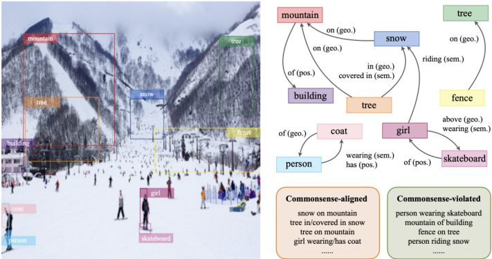
Figure 1. Example scene graph. Each edge represents a predicted relationship under a geometric, possessive, or semantic supercategory, and it can be either commonsense-aligned or violated.
图 1: 示例场景图。每条边代表在几何、所属或语义超类别下预测的关系,可以是符合常识或违背常识的。
Although an advanced scene graph generation model may achieve good performance indicated by its high recall scores [43, 60], it may produce a wide range of unreasonable relationships that are unlikely to occur in the real world, such as ”bunny jumping plate”, even with a high confidence. Recent advances in large language models (LLMs) [1, 4–6, 20, 61, 63] and vision-language mod- els (VLMs) [40, 41, 44, 49, 53, 66] now enables machines to perform commonsense reasoning [7, 67, 82]. Therefore, we incorporate LLMs or VLMs into the system to critique the output of a scene graph generation model, removing predicates that are not accord with common sense intuitions.
虽然先进的场景图生成模型可能通过高召回率分数展现出优异性能[43, 60],但它仍可能生成大量现实中不太可能存在的荒谬关系(例如"兔子跳跃盘子"),即使这些预测具有高置信度。随着大语言模型[1, 4–6, 20, 61, 63]和视觉语言模型[40, 41, 44, 49, 53, 66]的最新进展,机器现已具备常识推理能力[7, 67, 82]。因此,我们将大语言模型或视觉语言模型集成到系统中,用于评估场景图生成模型的输出结果,剔除不符合常识直觉的谓词关系。
In this study, we present the HIErarchical Relation head and COMmonsense validation pipeline, HIERCOM. Comprehensive experimental results show that these straight forward, plug-and-play modules can substantially enhance the performance of existing scene graph generation models, often by a large margin. Improvements are observed across Recall $\ @k$ [43], mean Recall $\ @k$ [60], and zero-shot evaluation metrics. These two innovations enable even a simple baseline model to produce reliable, commonsense-aligned outcomes, and elevate state-of-the-art (SOTA) methods to new levels of performance. Furthermore, our findings reveal that language models, regardless of their scale or whether they are augmented with vision capabilities, perform robustly in commonsense validation tasks. This consistency in strength makes our algorithms more accessible, allowing the community to deploy HIERCOM with just a small-scale, language-only model on local devices for efficient scene graph generation.
在本研究中,我们提出了层次化关系头(HIErarchical Relation head)与常识验证流程(COMmonsense validation pipeline)相结合的HIERCOM框架。综合实验结果表明,这些即插即用的简洁模块能显著提升现有场景图生成模型的性能,且提升幅度往往很大。改进体现在召回率$\ @k$ [43]、平均召回率$\ @k$ [60]以及零样本评估指标等多个维度。这两项创新使得即使简单基线模型也能产生可靠且符合常识的结果,并将最先进(SOTA)方法的性能推向新高度。此外,我们的研究发现:无论语言模型的规模大小或是否具备视觉能力,它们在常识验证任务中均表现稳健。这种稳定的性能使我们的算法更具普适性,社区只需在本地设备部署小型纯语言模型,即可利用HIERCOM实现高效的场景图生成。
2. Related Work
2. 相关工作
Scene graph generation with hierarchical information Neural Motifs [76], as an early work, analyzes the Visual Genome [28] dataset and divide the 50 most frequent re- lations into 3 super-categories: geometric, possessive, and semantic, as detailed in Figure 5. Unfortunately, it does not further utilize the super-categories it identifies. Our work follows their definitions and fully utilizes this hierarchical structure. Besides, HC-Net [54] investigates hierarchical contexts, rather than the relations. [47] studies the fine-grained relations and explores different usage of each predicate in practice. GPS-Net [39] focuses on understanding the relative priority of the graph nodes. CogTree [73] and HML [13] focus on automatically building a tree structure from coarse to fine-grained levels, while relations in our work are clustered by their semantic meanings either manually [76] or automatically using token embeddings.
场景图生成的层次信息利用
Neural Motifs [76] 作为早期研究,分析了 Visual Genome [28] 数据集并将 50 种最频繁的关系划分为 3 个超类别:几何关系、所属关系和语义关系(详见图 5)。遗憾的是,该研究未进一步利用其识别的超类别。我们的工作沿用其定义并充分挖掘了这一层次结构。此外,HC-Net [54] 研究的是层次化上下文而非关系本身。[47] 探索了细粒度关系及不同谓词的实际应用差异。GPS-Net [39] 专注于理解图节点的相对优先级。CogTree [73] 和 HML [13] 致力于从粗粒度到细粒度自动构建树状结构,而本研究中的关系聚类则通过人工标注 [76] 或基于 token 嵌入的自动方式按语义进行划分。
Scene graph generation with foundation models ELEGANT [81] leverages LLMs to propose potential relation candidates based on common sense and utilizes BLIP2 [30], a visual question answering model, for validation. [71] uses CLIP [50] to verify extracted triplets from knowledge bases, and RECODE [32] further aids CLIP with visual cues from LLMs. [45] prompts VLMs to generate scene graphs in JSON formats. VLM4SGG [26] and other works [37, 72, 83] allow language supervisions for weakly supervised generation, and [18,34,74,80] further extend the scope to open vocabularies.
基于基础模型的场景图生成
ELEGANT [81] 利用大语言模型 (LLM) 根据常识提出潜在关系候选,并借助视觉问答模型 BLIP2 [30] 进行验证。[71] 使用 CLIP [50] 验证从知识库提取的三元组,RECODE [32] 则通过大语言模型提供的视觉线索增强 CLIP 的效能。[45] 引导视觉语言模型 (VLM) 生成 JSON 格式的场景图。VLM4SGG [26] 及其他研究 [37, 72, 83] 支持通过语言监督实现弱监督生成,[18,34,74,80] 进一步将适用范围扩展至开放词汇领域。
Other scene graph generation methods Scene graph generation was initially proposed in [22, 43]. Many approaches tackle the problem from the perspective of graphical neural networks [10, 23, 39, 56, 64, 68, 70, 75] or recurrent networks [11, 15, 68, 76] to integrat global contexts. In recent years, [24] shifts the iterative message passing to transformers. EGTR [19] extracts relations from selfattention layers of the DETR [8] decoder. BGT-Net [15] and RTN [27] integrates two transformers for objects and edges, respectively. RelTR [12] and SSR-CNN [62] further extends the notions to triplets. [57] offers an energy-based framework. [69] establishes a conditional random field to model the distribution of objects and relations. [59] aims to remove the bias from prediction via total direct effects.
其他场景图生成方法
场景图生成最初由[22, 43]提出。许多方法从图神经网络[10, 23, 39, 56, 64, 68, 70, 75]或循环网络[11, 15, 68, 76]的角度出发,整合全局上下文。近年来,[24]将迭代消息传递转向Transformer架构。EGTR[19]从DETR[8]解码器的自注意力层提取关系。BGT-Net[15]和RTN[27]分别用两个Transformer处理物体和边。RelTR[12]与SSR-CNN[62]进一步将概念扩展到三元组。[57]提出了基于能量的框架。[69]建立条件随机场建模物体与关系的分布。[59]通过总直接效应消除预测偏差。
Furthermore, there are a series of works paying specific attention to the long-tailed distributions of relations [13, 16, 31, 35, 36, 42, 47, 59, 73, 74, 77]. Most works sacrifice $\mathbf R\ @k$ [43] for $\mathrm{mR}@k$ [60] scores. However, our work presents plug-and-play approaches that are model-agnostic, so it can incorporate with those models - specifically designed for reducing imbalance - to improve both their $\mathbf R\ @k$ and $\mathrm{mR}@k$ scores simultaneously. We show experiments in Section 4.4 and the detailed histogram in Figure 5.
此外,还有一系列研究专门关注关系的长尾分布 [13, 16, 31, 35, 36, 42, 47, 59, 73, 74, 77]。大多数工作以牺牲 $\mathbf R\ @k$ [43] 为代价来提升 $\mathrm{mR}@k$ [60] 分数。然而,我们的工作提出了即插即用且与模型无关的方法,因此可以与那些专门为减少不平衡而设计的模型结合使用,从而同时提高它们的 $\mathbf R\ @k$ 和 $\mathrm{mR}@k$ 分数。我们在第4.4节展示了实验,并在图5中提供了详细的直方图。
3. Scene Graph Construction
3. 场景图构建
A scene graph $G={V,E}$ is a graphical representation of an image. The set of vertices $V$ consists of $n$ object instances, including their bounding boxes and labels. The set of edges $E$ consists of one or more relationships $\mathbf{r}$ , if any.
场景图 $G={V,E}$ 是图像的图形化表示。顶点集 $V$ 由 $n$ 个对象实例构成,包含其边界框和标签。边集 $E$ 包含一个或多个关系 $\mathbf{r}$(若存在)。
This section first introduces a standalone baseline model with a better evaluation flexibility. It then describe the proposed hierarchical relation head and commonsense validation pipeline, which are designed as plug-and-play modules that can continue enhancing existing SOTA scene graph generation methods to new levels of performance.
本节首先介绍一个具有更好评估灵活性的独立基线模型,随后阐述所提出的分层关系头模块和常识验证流程。这些组件被设计为即插即用模块,能够持续提升现有最先进场景图生成方法的性能至新高度。
3.1. Baseline model
3.1. 基线模型
We propose a simple yet strong baseline model that adapts the widely-used two-stage design [15, 39, 68, 70, 76]. It starts with a Detection Transformer (DETR) [8] as the object detector with a ResNet-101 backbone [17]. Its transformer encoder [8, 65] can contextual ize image features $\pmb{I}\in\mathbb{R}^{h\times s\times t}$ with global information at an earlier stage of the scene graph generation pipeline. Here, $h$ is the hidden channels, while $s$ and $t$ denote the spatial dimensions. Its decoder outputs a set of object bounding boxes and labels in parallel. We also integrate MiDaS [51] to estimate a depth map $D\in\mathbb{R}^{s\times t}$ from each single image, which will be concatenated with I as I′ ∈ R(h+1)×s×t.
我们提出了一种简单但强大的基线模型,该模型采用了广泛使用的两阶段设计[15, 39, 68, 70, 76]。它以 Detection Transformer (DETR) [8] 作为目标检测器,并采用 ResNet-101 主干网络[17]。其 Transformer 编码器[8, 65]能够在场景图生成流程的早期阶段,利用全局信息对图像特征 $\pmb{I}\in\mathbb{R}^{h\times s\times t}$ 进行上下文建模。其中,$h$ 表示隐藏通道数,$s$ 和 $t$ 表示空间维度。解码器并行输出一组物体边界框和标签。我们还集成了 MiDaS [51] 从每张单张图像中估计深度图 $D\in\mathbb{R}^{s\times t}$,该深度图将与 I 拼接为 I′ ∈ R(h+1)×s×t。
The model computes hidden embeddings for both the subject and object instances, separately, to overcome possible overlaps between them and maintain their relative spatial locations. These embeddings are obtained by dotmultiplying their respective bounding boxes $M_{i},M_{j}\in$ $\mathbb{R}^{s\times t}$ with $\pmb{I}^{\prime}$ , resulting in two feature tensors $\pmb{I}{i}^{\prime},\pmb{I}{j}^{\prime}\in$ R(h+1)×s×t. To address the directional nature of relationships, $\pmb{I}{i}^{\prime}$ and $\pmb{I}{j}^{\prime}$ are concatenated in both possible directions as $\boldsymbol{I}{i j}^{\prime}$ and $\bar{\pmb{I_{j i}^{\prime}}}\in\mathbb{R}^{2\cdot(h+1)\times s\times t}$ . The concatenated tensors are then fed separately into subsequent linear layers as $X_{i j}$ and $\pmb{X}{j i}\in\mathbb{R}^{d}$ , and the classification head will finally estimate the relations $\mathbf{r}{i j}$ and $\mathbf{r}_{j i}$ , as shown in Equation 1.
该模型分别计算主体和客体实例的隐藏嵌入,以克服它们之间可能的重叠并保持其相对空间位置。这些嵌入通过将各自的边界框 $M_{i},M_{j}\in$ $\mathbb{R}^{s\times t}$ 与 $\pmb{I}^{\prime}$ 进行点乘得到,生成两个特征张量 $\pmb{I}{i}^{\prime},\pmb{I}{j}^{\prime}\in$ R(h+1)×s×t。为了解决关系的方向性,$\pmb{I}{i}^{\prime}$ 和 $\pmb{I}{j}^{\prime}$ 按两种可能的方向拼接为 $\boldsymbol{I}{i j}^{\prime}$ 和 $\bar{\pmb{I_{j i}^{\prime}}}\in\mathbb{R}^{2\cdot(h+1)\times s\times t}$。拼接后的张量分别输入后续的线性层,得到 $X_{i j}$ 和 $\pmb{X}{j i}\in\mathbb{R}^{d}$,分类头最终估计关系 $\mathbf{r}{i j}$ 和 $\mathbf{r}_{j i}$,如公式1所示。
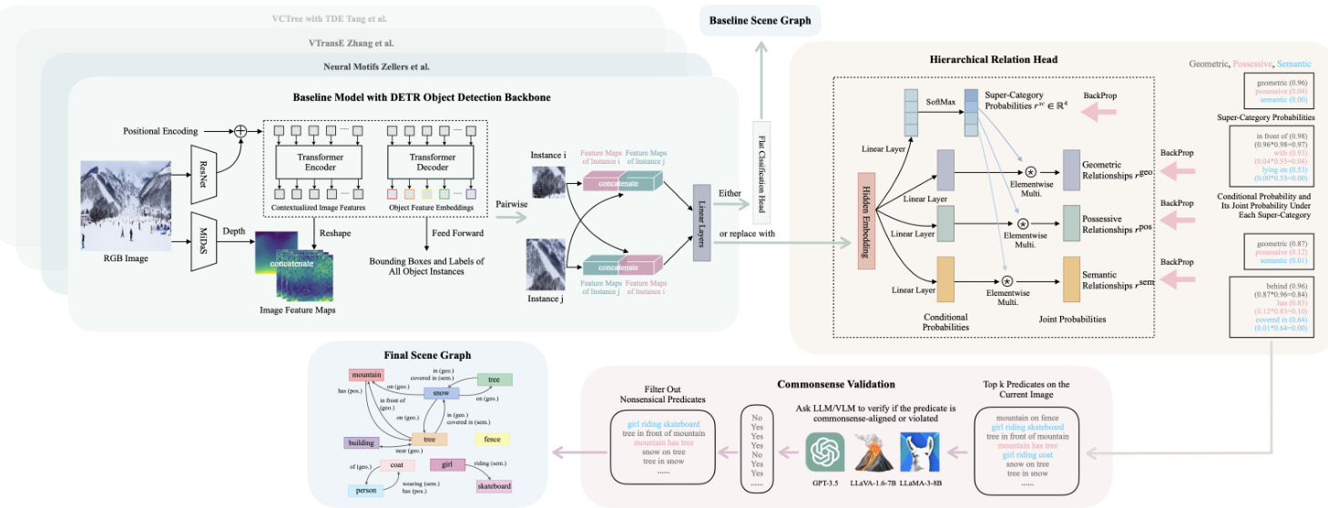
Figure 2. This diagram provides an overview of HIERCOM. The core components of HIERCOM are the hierarchical relation head and the commonsense validation pipeline, both of which are model-agnostic plug-and-play modules, suitable for integration with a variety of baseline scene graph generation models that have a conventional flat classification head. Specifically, the hierarchical relation head is designed to replace this flat layer, jointly estimating relation super-categories and more granular relations within each category. Additionally, the diagram depicts a baseline scene graph generation model: an RGB image is the input, supplemented by an estimated depth map. Using the DETR object detector, the model generates feature maps, object labels, and bounding boxes. Relationship estimation between each pair of instances occurs in two separate passes - to account for directional relationships - first assuming one instance as the subject and then the other. Subsequently, the commonsense validation pipeline leverages an LLM or VLM - which can have a small size - to filter out commonsense-violating predicates, thus refining the final scene graphs to include more predicates that align with the common sense.
图 2: 本图展示了HIERCOM的总体框架。该系统的核心组件是分层关系头(hierarchical relation head)和常识验证流程(commonsense validation pipeline),这两个模块均采用与模型无关的即插即用设计,可适配各类配备传统扁平分类头的场景图生成基线模型。具体而言,分层关系头用于替代原有扁平分类层,通过联合预测关系超类别及各超类别下的细粒度关系实现层级化建模。图中同时展示了基线场景图生成模型的工作流程:以RGB图像为输入,辅以估计的深度图;通过DETR目标检测器生成特征图、物体标签及边界框;每对实例的关系预测分两次独立计算(以处理方向性关系)——先假设一个实例为主语再假设另一个实例为主语。最后,常识验证流程调用轻量化的大语言模型或视觉语言模型,过滤违反常识的谓词,从而优化最终场景图使其包含更多符合常识的谓词。
$$
\boldsymbol{r}{i j},\boldsymbol{r}{j i}=\mathrm{SoftMax}{X_{i j}^{\top}W},\mathrm{SoftMax}{X_{j i}^{\top}W}
$$
$$
\boldsymbol{r}{i j},\boldsymbol{r}{j i}=\mathrm{SoftMax}{X_{i j}^{\top}W},\mathrm{SoftMax}{X_{j i}^{\top}W}
$$
where $W$ is a learnable parameter tensor of the linear layer.
其中 $W$ 是线性层的可学习参数张量。
3.2. Hierarchical relation head
3.2. 层次关系头
Inspired by the Bayes’ rule, the hierarchical relation head is designed to replace the by-default flat classification head in Equation 1. It predicts the following four items:
受贝叶斯规则启发,层级关系头被设计用来替代公式1中的默认扁平分类头。它预测以下四项:
$$
\begin{array}{r}{\begin{array}{l}{{r_{i j}^{\mathrm{sc}}=\mathrm{SoftMax}{X_{i j}^{\top}W^{\mathrm{sc}}}}}\ {{r_{i j}^{\mathrm{geo}}=\mathrm{SoftMax}{X_{i j}^{\top}W^{\mathrm{geo}}}\cdot r_{i j}^{\mathrm{sc}}[0]}}\ {{r_{i j}^{\mathrm{pos}}=\mathrm{SoftMax}{X_{i j}^{\top}W^{\mathrm{pos}}}\cdot r_{i j}^{\mathrm{sc}}[1]}}\ {{r_{i j}^{\mathrm{sem}}=\mathrm{SoftMax}{X_{i j}^{\top}W^{\mathrm{sem}}}\cdot r_{i j}^{\mathrm{sc}}[2]}}\end{array}}\end{array}
$$
$$
\begin{array}{r}{\begin{array}{l}{{r_{i j}^{\mathrm{sc}}=\mathrm{SoftMax}{X_{i j}^{\top}W^{\mathrm{sc}}}}}\ {{r_{i j}^{\mathrm{geo}}=\mathrm{SoftMax}{X_{i j}^{\top}W^{\mathrm{geo}}}\cdot r_{i j}^{\mathrm{sc}}[0]}}\ {{r_{i j}^{\mathrm{pos}}=\mathrm{SoftMax}{X_{i j}^{\top}W^{\mathrm{pos}}}\cdot r_{i j}^{\mathrm{sc}}[1]}}\ {{r_{i j}^{\mathrm{sem}}=\mathrm{SoftMax}{X_{i j}^{\top}W^{\mathrm{sem}}}\cdot r_{i j}^{\mathrm{sc}}[2]}}\end{array}}\end{array}
$$
where $\cdot$ represents the scalar product, $\pmb{r}{i j}^{\mathrm{sc}}\in\mathbb{R}^{4}$ represents the probabilities of the three relation super-categories plus the background class, and ${\pmb{r}{i j}^{c}|c\in[\mathrm{geo,pos,sem}]}$ are the joint probabilities under each super-category. Same for $\mathbf{r}_{j i}$ in the other direction.
其中 $\cdot$ 表示标量积,$\pmb{r}{i j}^{\mathrm{sc}}\in\mathbb{R}^{4}$ 表示三个关系超类别加上背景类的概率,${\pmb{r}{i j}^{c}|c\in[\mathrm{geo,pos,sem}]}$ 是每个超类别下的联合概率。另一方向的 $\mathbf{r}_{j i}$ 同理。
To train the hierarchical relation head, we apply crossentropy losses to all four terms in Equation 2-5. In addition, we use a supervised contrastive loss [25] to minimize the distances in embedding space within the same relation class (set $P(i j)$ and maximize those from different relationship classes (set $N(i j)$ .
为训练层次关系头,我们对公式2-5中的全部四项应用交叉熵损失。此外,采用监督对比损失[25]来最小化嵌入空间中同类关系(集合$P(ij)$)的距离,同时最大化不同关系类(集合$N(ij)$)的距离。
where the underlined quantities denote ground truth values from the dataset, $\mathcal{L}{\mathrm{sup.rel}}$ is the loss for relation supercategories, $\mathcal{L}{\mathrm{sub.rel}}$ is the loss for detailed relationships, $\mathcal{L}_{\mathrm{contrastive}}$ is the contrastive loss, and $\tau$ is the temperature. 1 is an indicator function, meaning that we back-propagate the losses only to the relations under target super-categories.
其中带下划线的量表示数据集中的真实值,$\mathcal{L}{\mathrm{sup.rel}}$ 是关系超类别的损失,$\mathcal{L}{\mathrm{sub.rel}}$ 是详细关系的损失,$\mathcal{L}_{\mathrm{contrastive}}$ 是对比损失,$\tau$ 是温度参数。1 是一个指示函数,意味着我们仅将损失反向传播到目标超类别下的关系。
The model yields three predicates for each edge, one from each disjoint super-category, maintaining the exclusivity among relations within the same super-category. All three predicates from each edge will participate in the confidence ranking. Because there will be three times more candidates, we are not trivially relieving the graph constraints [48, 76] to make the task simpler.
该模型为每条边生成三个谓词,分别来自三个互不相交的超类别,确保同一超类别内的关系保持互斥性。每条边的三个谓词都将参与置信度排名。由于候选数量增加了三倍,我们并未简单放宽图约束 [48, 76] 来降低任务难度。
It is often the case that two predicates from disjoint super-categories of the same edge will appear within the top $k$ predictions, providing different interpretations of the edge. This design leverages the super-category probabilities to guide the network’s attention toward the appropriate conditional output heads, enhancing the interpret ability and performance of the system.
同一边缘的不同超类别中的两个谓词常会同时出现在前 $k$ 个预测结果中,从而对该边缘提供不同的解释。这一设计利用超类别概率来引导网络关注适当的条件输出头,从而提升系统的可解释性和性能。
3.3. Commonsense validation
3.3. 常识验证
Language or vision-language models can critique output predictions of a scene graph generation algorithm and select those that align with common sense. In our settings, we intend to only leverage open-sourced, small-scale language models like LLaMA-3-8B [63] or small vision-language models like LLaVA-1.6-7B [40] to handle this complex graphical task. This choice is motivated by the potential interests in applying these algorithms on local devices, particularly within the robotics community [2, 3, 38, 46], where computations and space are crucial considerations. We also provide a comparison with larger, commercial alternatives like GPT-3.5 [6] in Section 4.
语言或视觉-语言模型能够评判场景图生成算法的输出预测,并筛选出符合常识的结果。在我们的设定中,我们仅计划利用开源的小规模语言模型(如LLaMA-3-8B [63])或小型视觉-语言模型(如LLaVA-1.6-7B [40])来处理这一复杂的图形任务。这一选择源于将这些算法应用于本地设备(尤其是机器人领域 [2, 3, 38, 46])的潜在需求,其中计算资源和存储空间是关键考量因素。我们还在第4节中提供了与GPT-3.5 [6]等更大规模商业替代方案的对比。
By deploying small, open-sourced models, we harness their abilities as a commonsense validator, rather than asking them to generate a scene graph from scratch, which could be more challenging. We query such a foundation model on whether each of the top m-n most confident predicates identified per image is reasonable or not using the prompts in Figure 3. This validation process aims to filter out predictions with high confidence but violate the basic commonsense in the physical world.
通过部署小型开源模型,我们将其作为常识验证器来利用其能力,而不是要求它们从头生成场景图(这更具挑战性)。我们使用图3中的提示词,针对每张图像识别出的前m-n个最置信谓词,逐一查询基础模型以判断其合理性。该验证流程旨在过滤掉那些置信度高但违反物理世界基本常识的预测。
3.4. Seamless integration with existing frameworks
3.4. 与现有框架的无缝集成
Figure 2 illustrates how the proposed (1) hierarchical relation head and (2) commonsense validation pipeline can be easily integrated as plug-and-play modules into not only our baseline model but also other existing SOTA scene graph generation algorithms. Specifically, the hierarchical relation head can replace the final linear layer in the classifica- tion heads of these models, refining the process of relation- ship classification. Subsequently, the predicted triplets can undergo the commonsense validation pipeline, eliminating nonsensical ones in the final outputs.
图 2: 展示了所提出的 (1) 层次化关系头 (hierarchical relation head) 和 (2) 常识验证流程 (commonsense validation pipeline) 如何作为即插即用模块,不仅可集成至我们的基线模型,还能兼容其他现有 SOTA 场景图生成算法。具体而言,层次化关系头可替换这些模型分类头中的最终线性层,从而优化关系分类过程。随后,预测的三元组将经过常识验证流程,最终输出中会剔除不符合常识的无效结果。
4. Experiments
4. 实验
4.1. Datasets and evaluation metrics
4.1. 数据集和评估指标
Our experiments are conducted on Visual Genome [28] and OpenImage V6 [29] datasets, following the same preprocessing procedures and splits in [33, 68]. On Visual Genome, we select the top 150 object labels and 50 relations, resulting in $75.7k$ training and $32.4k$ testing images. We adopt Recall $\ @k$ $({\mathsf{R@}}k)$ and mean Recall $\ @k$ $(\mathrm{mR}@k)$ [43, 60]. $\mathbf R\ @k$ measures the recall within the top $k$ most confident predicates per image, while $\mathrm{mR@\mathcal{k}}$ computes the average across all relation classes. Zeroshot recall $(\mathtt{z s R@k})$ [59] calculates $\mathbf{R}\ @k$ for the triplets that only appear in the testing dataset. We conduct three tasks: (1) Predicate classification (PredCLS) predicts re
我们的实验在Visual Genome [28]和OpenImage V6 [29]数据集上进行,遵循与[33, 68]相同的预处理流程和数据划分。在Visual Genome中,我们筛选了前150个物体标签和50种关系,最终得到$75.7k$张训练图像和$32.4k$张测试图像。采用召回率$\ @k$ $({\mathsf{R@}}k)$和平均召回率$\ @k$ $(\mathrm{mR}@k)$ [43, 60]作为评估指标。$\mathbf R\ @k$衡量每张图像前$k$个最高置信度谓词的召回率,而$\mathrm{mR@\mathcal{k}}$计算所有关系类别的平均值。零样本召回率$(\mathtt{z s R@k})$ [59]则针对仅出现在测试数据集中的三元组计算$\mathbf{R}\ @k$。我们开展了三项任务:(1) 谓词分类(PredCLS)预测...
meta-llama-3-8b-instruct (language-only model, one inference per triplet)
meta-llama-3-8b-instruct (纯语言模型,每个三元组推理一次)
llava-v1.6-vicuna-7b (vision-language model, one inference per triplet)
llava-v1.6-vicuna-7b (视觉语言模型,每个三元组推理一次)
Image:[IMAGE]
图: [IMAGE]
Prompt:"In this image,canyou finda'?Answer only'Yes'orNo'"
提示:"在此图像中,你能找到一个'吗?只需回答'是'或'否'"
gpt-3.5-turbo (language-only model, one inference per graph)
gpt-3.5-turbo (纯语言模型,每个图表一次推理)
Role:"System",Content:"Your task is tofilter out invalid triplets."
角色: "系统", 内容: "你的任务是过滤无效的三元组。"
Role:"User",Content:"Given the following list,check each triplet onebyone andexplain. Ifit violate the commonsense or is impossible in the physical world,say'No'Otherwise,say'Yes' Here is the list:0..0
角色:"用户",内容:"给定以下列表,逐一检查每个三元组并解释。如果违反常识或在物理世界中不可能,回答'否';否则回答'是'。列表如下:0..0"
Role:"Assistant",Content:[Model Outputs]
角色:"助手",内容:[模型输出]
Role:"User"Content:"Summarize your answers as a Python list of only Yes and No'uchas $\mathit{\Gamma}{\mathit{i}}\mathit{Y}{e s}$ Yes,No,Yes,whose length must beequalto the number of triplets mentioned Do not include any other words."
角色:"用户"
内容:"将你的回答总结为一个仅包含 Yes 和 No 的 Python语言 列表,例如 $\mathit{\Gamma}{\mathit{i}}\mathit{Y}{e s}$ Yes, No, Yes,其长度必须与提到的三元组数量相等。不要包含任何其他词语。"
Figure 3. Prompt engineering across different foundation models, where $\because{}^{,}$ is a placeholder for a triplet written in string, such as “girl riding skateboard”. For LLaMA-3-8B, which lacks the vision capability, we employ three distinct prompts for each of the top m-n predicted triplets, and collect a majority vote on whether each triplet makes sense to enhance the robustness. In contrast, LLaVA-1.6-7B is prompted to verify whether each of the top $m{-}n$ predicted triplets actually appears in the image. Since GPT-3.5 is much larger than LLaMA-3-8B with better instruction-following capabilities, we use a single prompt to evaluate all the top $m{-}n$ predicates in the (sub)graph of each image, and collect a list of ‘Yes’ or ‘No’ responses simultaneously with a higer efficiency.
图 3: 不同基础模型间的提示工程,其中 $\because{}^{,}$ 表示用字符串书写的三元组占位符,例如"girl riding skateboard"。对于缺乏视觉能力的LLaMA-3-8B,我们为每个top m-n预测三元组设计三种不同提示,并通过多数表决机制判断每个三元组是否合理以增强鲁棒性。相比之下,LLaVA-1.6-7B被要求验证每个top $m{-}n$预测三元组是否真实出现在图像中。由于GPT-3.5规模远大于LLaMA-3-8B且具有更优的指令跟随能力,我们使用单一提示来评估每张图像(子)图中所有top $m{-}n$谓词,并以更高效率同步收集"Yes"或"No"的响应列表。
lations with ground-truth bounding boxes and labels. (2) Scene graph classification (SGCLS) only assumes known bounding boxes. (3) Scene graph detection (SGDET) has no prior knowledge of objects, while predicted and target boxes should have an IOU of at least 0.5 [43].
与真实边界框和标签的关系。 (2) 场景图分类(SGCLS)仅假设已知边界框。 (3) 场景图检测(SGDET)对物体没有先验知识,而预测框与目标框的IOU需至少达到0.5 [43]。
On OpenImage V6, we keep 601 object labels and 30 relations, resulting in around $53.9k$ training and $3.2k$ testing images. We adopt its standard metrics: Recall $\ @50$ , the weighted mean average precision of relationships wm $\mathrm{{1AP{rel}}}$ and phrases $\mathrm{wmAP_{phr}}$ , and the final score $=0.2\cdot R{\widehat{\ @}}50+$ $0.4\cdot\mathrm{wmAP_{rel}}+0.4\cdot\mathrm{wmAP_{phr}}$ , as detailed in [79].
在OpenImage V6数据集上,我们保留了601个物体标签和30种关系,最终得到约$53.9k$张训练图像和$3.2k$张测试图像。采用其标准评估指标:召回率$\ @50$、关系加权平均精度$\mathrm{wmAP_{rel}}$和短语加权平均精度$\mathrm{wmAP_{phr}}$,最终得分计算公式为$0.2\cdot R{\widehat{\ @}}50+0.4\cdot\mathrm{wmAP_{rel}}+0.4\cdot\mathrm{wmAP_{phr}}$,具体细节见[79]。
4.2. Numerical results
4.2. 数值结果
Table 1 highlights the main experimental results. The proposed hierarchical relation head and commonsense validation pipeline are model-agnostic, so we compare the performance on multiple backbone models with and without integrating the proposed modules. Our comparative analysis demonstrates that such a simple incorporation, in almost all cases, enhance the performance by a large margin across all three tasks on both $\mathbf{R}\ @k$ [43] and $\mathrm{mR@\mathcal{k}}$ [60] scores, affirming the promising of our approach. Zero-shot results in Table 5 also support the same conclusion.
表1: 主要实验结果对比。我们提出的层次化关系头模块和常识验证流程与模型无关,因此对比了多个骨干模型在集成/未集成该模块时的性能表现。对比分析表明,这种简单集成在几乎所有情况下都能显著提升三项任务在$\mathbf{R}\ @k$[43]和$\mathrm{mR@\mathcal{k}}$[60]指标上的表现,验证了方法的有效性。表5中的零样本实验结果也支持相同结论。
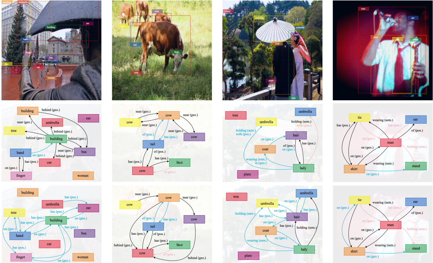
Figure 4. Illustration of generated scene graphs on predicate classification. All examples are from the testing dataset of Visual Genome. The first row displays images and objects, while the second row displays the final scene graphs. The third row shows an ablation without commonsense validation. For each image, we display the top 10 most confident predictions, and each edge is annotated with its relation label and super-category. Meanwhile, it is possible for an edge to have multiple predicted relationships, but they must come from disjoint super-categories. In this figure, pink edges are true positives in the dataset. Blue edges represent incorrect edges based on our observations Interestingly, all the black edges are reasonable predictions we believe but not annotated, which should not be regarded as false positives.
图 4: 谓词分类生成场景图示例。所有样本均来自Visual Genome测试集。首行展示图像及物体,次行呈现最终场景图,第三行为移除常识验证的消融实验。每张图像仅显示置信度最高的10个预测结果,每条边均标注关系类别及父类。需注意,单条边可能对应多个预测关系,但这些关系必须来自互斥的父类。图中粉色边代表数据集中的真实正例,蓝色边为基于观察认定的错误边。有趣的是,所有黑色边虽未标注但均属合理预测,不应视为假阳性结果。
4.3. Visual results
4.3. 可视化结果
Figure 4 showcases some predicted scene graphs, which include their top 10 most confident predicates. The second row displays final scene graphs and the third row shows an ablation without commonsense validation.
图 4: 展示了一些预测的场景图,包含其置信度最高的前10个谓词。第二行显示最终场景图,第三行展示了未进行常识验证的消融实验结果。
The commonsense validation pipeline successfully efficiently reduces many unreasonable predicates that would otherwise have appeared on top of the confidence ranking, for example, it removes the predicate “tree has hand” in the left-most image from its initial prediction. However, in the right-most image, the LLM fails at “shirt on stand”, a possible relation in the real world but unrelated to the scene. Furthermore, it is important to note that there are numerous valid predictions aligned with intuitions that are not annotated; these are marked in black, whose number significantly exceeds the number of pink edges representing true positives according to dataset annotations. This discrepancy highlights the sparse nature of the dataset’s annotations. Besides, all blue edges are incorrect predictions based on both the original dataset annotations and our observations.
常识验证流程成功高效地减少了大量本会出现在置信度排名前列的不合理谓词,例如它移除了最左侧图像中初始预测的谓词"树有手"。然而在最右侧图像中,大语言模型未能正确识别"衬衫挂在支架上"这一关系——虽然该关系在现实世界中可能存在,但与当前场景无关。值得注意的是,存在大量符合直觉却未被标注的有效预测(以黑色标记),其数量远超数据集中标注为真阳性的粉色边。这种差异凸显了数据集标注的稀疏性。此外,所有蓝色边都是基于原始数据集标注和我们观察得出的错误预测。
Still, our model learns rich relational information even being trained from incomplete annotations. We strongly believe that creating an extensive set of predicates is beneficial for practical scene understanding.
尽管如此,我们的模型即使从未完整标注的数据中训练,也能学习到丰富的关系信息。我们坚信构建广泛的谓词集对实际场景理解大有裨益。
4.4. More results on the hierarchical relation head
4.4 层次关系头的更多结果
Training details The baseline model is trained using a batch size of 12 for three epochs on Visual Genome or one epoch on OpenImage V6, using two NVIDIA V100 GPUs with 32GB memory. We use an SGD optimizer with a learning rate of 1e-5 and a step scheduler that decreases $l r$ to 1e-6 at the third epoch. We take the DETR backbone from [33] pretrained on the same training dataset and freeze it in our experiments. The model has a size of roughly 1055MB and takes an average of 0.2 seconds on single-image inference. Our plug-and-play experiments are build upon the code framework in [58, 59]. We keep training parameters the same, except for learning rates, and retrain all models from scratch with the hierarchical relation head replacing the final linear layer of the original classification head.
训练细节
基线模型在 Visual Genome 数据集上训练 3 个周期或在 OpenImage V6 数据集上训练 1 个周期,批量大小为 12,使用两块 32GB 显存的 NVIDIA V100 GPU。我们采用学习率为 1e-5 的 SGD 优化器,并配合阶梯式调度器在第三个周期将 $l r$ 降至 1e-6。DETR 主干网络来自 [33] 的预训练模型(基于相同训练数据集),实验中保持冻结状态。模型大小约为 1055MB,单图推理平均耗时 0.2 秒。即插即用实验基于 [58, 59] 的代码框架实现,除学习率外保持其他训练参数不变,并通过用分层关系头替换原始分类头的最终线性层来从头训练所有模型。
Table 1. This table showcases the main experimental results, presenting Recall $\ @k$ and mean Recall $\ @k$ scores from the testing dataset of Visual Genome. We integrate the proposed hierarchical relation head and commonsense validation pipeline into existing scene graph generation algorithms, comparing the performance both with and without these plug-and-play modules. Improvements are evident, with higher scores highlighted in bold, demonstrating the effectiveness of our approaches across a variety of baseline models. For these evaluations, the commonsense validation employs LLaVA-1.6-7B, while results utilizing other foundation models are detailed in Table 7.
表 1: 该表展示了在Visual Genome测试数据集上的主要实验结果,呈现了召回率$\ @k$和平均召回率$\ @k$的分数。我们将提出的分层关系头和常识验证流程集成到现有场景图生成算法中,比较了包含与不包含这些即插即用模块的性能差异。改进效果显著,加粗显示的高分证明了我们的方法在各种基线模型上的有效性。在这些评估中,常识验证使用了LLaVA-1.6-7B,而使用其他基础模型的结果详见表7。
| 方法 | PredCLS R@20 | R@50 | R@100 | SGCLS R@20 | R@50 | R@100 | SGDET R@20 | R@50 | R@100 |
|---|---|---|---|---|---|---|---|---|---|
| IMP [68] | - | 44.8 | 53.1 | - | 21.7 | 24.4 | - | 3.4 | 4.2 |
| HC-Net [54] | 59.6 | 66.4 | 68.8 | 34.2 | 36.6 | 37.3 | 22.6 | 28.0 | 31.2 |
| GPS-Net [39] | 60.7 | 66.9 | 68.8 | 36.1 | 39.2 | 40.1 | 22.6 | 28.4 | 31.7 |
| BGT-Net [15] | 60.9 | 67.3 | 68.9 | 38.0 | 40.9 | 43.2 | 23.1 | 28.6 | 32.2 |
| RelTR [12] | 63.1 | 64.2 | - | 29.0 | 36.6 | - | 21.2 | 27.5 | - |
| Baseline (ours) | 59.4 | 67.9 | 69.9 | 29.5 | 33.8 | 34.8 | 20.3 | 26.1 | 28.1 |
| Baseline+HIERCOM (ours) | 64.2 | 75.6 | 79.2 | 32.5 | 37.5 | 39.2 | 23.8 | 29.8 | 32.7 |
| NeuralMotifs [76] | 58.5 | 65.2 | 67.1 | 32.9 | 35.8 | 36.5 | 21.4 | 27.2 | 30.3 |
| NeuralMotifs+HIERCOM (ours) | 55.5 | 69.5 | 75.6 | 34.0 | 41.6 | 44.8 | 20.3 | 28.3 | 33.9 |
| VTransE [78] | 59.0 | 65.7 | 67.6 | 35.4 | 38.6 | 39.4 | 23.0 | 31.3 | 35.5 |
| VTransE+HIERCOM (ours) | 54.8 | 68.5 | 75.0 | 34.7 | 41.1 | 44.3 | 23.2 | 31.6 | 35.9 |
| VCTree [60] | 59.8 | 65.9 | 67.6 | 41.5 | 45.2 | 46.1 | 24.9 | 32.0 | 36.3 |
| VCTree+EBM[57] | 57.3 | 64.0 | 65.8 | 40.3 | 44.7 | 45.8 | 24.2 | 31.4 | 35.9 |
| VCTree+HIERCOM (ours) | 55.9 | 69.8 | 75.8 | 39.0 | 46.7 | 50.7 | 23.3 | 32.2 | 37.0 |
| VCTree+TDE[59] | 36.2 | 47.2 | 51.6 | 19.9 | 25.4 | 27.9 | 14.0 | 19.4 | 23.2 |
| VCTree+TDE+HIERCOM (ours) | 41.1 | 58.3 | 67.5 | 26.3 | 35.6 | 40.4 | 14.5 | 20.6 | 25.8 |
| 方法 | PredCLS mR@20 | mR@50 | mR@100 | SGCLS mR@20 | mR@50 | mR@100 | SGDET mR@20 | mR@50 | mR@100 |
|---|---|---|---|---|---|---|---|---|---|
| IMP [68] | 11.7 | 14.8 | 16.1 | 6.7 | 8.3 | 8.8 | 4.9 | 6.8 | 7.9 |
| GPS-Net [39] | 17.4 | 21.3 | 22.8 | 10.0 | 11.8 | 12.6 | 6.9 | 8.7 | 9.8 |
| BGT-Net [15] | 16.8 | 20.6 | 23.0 | 10.4 | 12.8 | 13.6 | 5.7 | 7.8 | 9.3 |
| RelTR [12] | 20.0 | 21.2 | - | 7.7 | 11.4 | - | 6.8 | 10.8 | - |
| Baseline (ours) | 12.1 | 15.1 | 15.8 | 5.8 | 7.2 | 7.8 | 3.2 | 4.6 | 5.5 |
| Baseline+HIERCOM (ours) | 17.7 | 23.9 | 26.7 | 9.1 | 11.7 | 12.9 | 4.9 | 8.2 | 10.0 |
| NeuralMotifs [76] | 11.7 | 14.8 | 16.1 | 6.7 | 8.3 | 8.8 | 4.9 | 6.8 | 7.9 |
| NeuralMotifs+HIERCOM (ours) | 16.3 | 25.1 | 30.6 | 9.8 | 14.6 | 17.3 | 5.7 | 8.5 | 10.6 |
| VTransE [78] | 11.6 | 14.7 | 15.8 | 6.7 | 8.2 | 8.7 | 3.7 | 5.0 | 6.0 |
| VTransE+HIERCOM (ours) | 17.9 | 26.6 | 32.2 | 10.3 | 15.1 | 17.8 | 6.7 | 9.6 | 12.0 |
| VCTree [60] | 13.1 | 16.5 | 17.8 | 8.5 | 10.5 | 11.2 | 5.3 | 7.2 | 8.4 |
| VCTree+EBM[57] | 14.2 | 18.2 | 19.7 | 10.0 | 12.5 | 13.5 | 5.7 | 7.7 | 9.1 |
| VCTree+HIERCOM (ours) | 17.6 | 26.3 | 31.8 | 11.8 | 16.9 | 20.0 | 5.8 | 8.7 | 11.1 |
| VCTree+TDE [59] | 17.3 | 24.6 | 28.0 | 9.3 | 12.9 | 14.8 | 6.3 | 8.6 | 10.5 |
| VCTree+TDE+HIERCOM (ours) | 20.3 | 29.1 | 35.5 | 14.3 | 20.0 | 23.7 | 7.3 | 10.7 | 13.7 |
Automatic clustering of the relation hierarchy This paragraph discusses an alternative design choice that automatic clusters the relation hierarchy. Instead of adhering to a manually defined hierarchy outlined in Neural Motifs [76], the clustering procedure does not necessarily require human involvement. For example, we can employ k-means, a classic unsupervised clustering technique, on pretrained embedding space to construct the relation hierarchy autonomously. Table 2 shows results using the CLIPText [50], GPT-2 [6], and BERT [14] embedding space by transforming relation labels as words into corresponding token embeddings. It turns out that CLIP performs the closest to the manual one in [76] with even higher $\mathrm{mR@k}$ scores, so CLIP could be utilized to generalize our idea to new datasets at any scale without the need for manual clustering.
关系层级的自动聚类
本段讨论了一种自动聚类关系层级的替代设计方案。与遵循Neural Motifs [76]中手动定义的层级结构不同,该聚类过程无需人工参与。例如,我们可以在预训练的嵌入空间上使用经典无监督聚类技术k-means,自主构建关系层级。表2展示了通过将关系标签转化为对应token嵌入,在CLIPText [50]、GPT-2 [6]和BERT [14]嵌入空间中的聚类结果。结果表明,CLIP的聚类效果最接近[76]中的人工标注层级,且$\mathrm{mR@k}$分数更高,因此可利用CLIP将我们的方案推广到任意规模的新数据集,而无需手动聚类。
Handling the long-tailed distribution We integrates the proposed modules into scene graph generation algorithms that are specifically tailored to address the long-tailed distribution of relation labels [31, 77]. Numerical results in Table 3 shows that our model-agnostic modules can continue raising their SOTA $\mathrm{mR}@k$ scores while simultaneously achieving even higher $\mathbf{R}\ @\mathbf{k}$ scores. Furthermore, the histograms in Figure 5 illustrates that we can gain further improvements on the labels at the tail of the distribution.
处理长尾分布
我们将提出的模块集成到专门用于解决关系标签长尾分布的场景图生成算法中 [31, 77]。表 3 中的数值结果表明,我们的模型无关模块可以持续提升其 SOTA $\mathrm{mR}@k$ 分数,同时实现更高的 $\mathbf{R}\ @\mathbf{k}$ 分数。此外,图 5 中的直方图显示,我们可以在分布尾部的标签上获得进一步的改进。
More ablation studies Table 4 details the impact of incorpora ting depth maps and the supervised contrastive loss
更多消融实验 表4详细说明了引入深度图和监督对比损失的影响

Figure 5. This figure compares the histograms between the original IETrans [77] and IETrans integrated with the proposed hierarchical relation head and commonsense validation, denoted as IETrans+HIERCOM. Different background colors for each relation label correspond to their super-category, as defined in [76]. While there is a slight decrease in performance for the head classes, continuing improvements are observed in the tail classes. Along with the data in Table 3, we show that our proposed methods not only elevate the $\mathrm{mR}@k$ scores but also maintain a good balance between the head and tail classes, simultaneously enhancing the $\mathbb{R}\ @k$ scores.
图 5: 该图对比了原始IETrans[77]与整合了分层关系头和常识验证的IETrans(记为IETrans+HIERCOM)的直方图分布。每个关系标签的不同背景色对应其超类别(定义见[76])。虽然头部类别性能略有下降,但尾部类别持续改善。结合表3数据可知,我们提出的方法不仅提升了$\mathrm{mR}@k$分数,同时保持了头尾类别的良好平衡,并提升了$\mathbb{R}\ @k$分数。
Table 2. This table presents ablation studies on different clustering methods used to structure the relation hierarchy. Results are evaluated on Baseline+HIER, i.e., without commonsense validation for the PredCLS task on Visual Genome. We compare man- ual clustering defined in [76] that categorizes relations into geometric, possessive, and semantic super-categories, with automatic clustering approaches. The latter ones transform relation labels into CLIP-Text, GPT-2, or BERT’s token embedding space and apply $\mathbf{k}$ -means clustering with $k=3$ . Results are comparably strong, suggesting that the proposed hierarchical relation head can be effectively generalized to new, larger datasets using automatic clustering methods, thus eliminating the need for manual effort.
表 2: 本表格展示了用于构建关系层次结构的不同聚类方法的消融研究。结果基于 Baseline+HIER 进行评估 (即在 Visual Genome 的 PredCLS 任务中未使用常识验证)。我们将 [76] 中定义的人工聚类 (将关系分为几何、所属和语义三大类) 与自动聚类方法进行对比。后者将关系标签转换为 CLIP-Text、GPT-2 或 BERT 的 token 嵌入空间,并应用 $\mathbf{k}$-means 聚类 ( $k=3$ )。结果表明各类方法性能相当,这说明所提出的层次化关系头可以通过自动聚类方法有效泛化到新的更大规模数据集,从而无需人工干预。
Table 3. This table illustrates the integration of the proposed hierarchical relation head with NICE [31] and IETrans [77], two state-of-the-art methods tailored to tackle the long-tailed distribution problem of relation labels. Typically, algorithms addressing long-tailed distributions may compromise $\mathbf{R}\ @k$ scores; however, results from the PredCLS task on Visual Genome demonstrate that incorporating the relation hierarchy not only continues to improve $\mathrm{mR}@k$ scores but also enhances their $\mathbb{R}\ @k$ simultaneously.
表 3: 该表展示了所提出的层次关系头与NICE [31]和IETrans [77]的集成效果,这两种方法专为解决关系标签的长尾分布问题而设计。通常,处理长尾分布的算法可能会牺牲$\mathbf{R}\ @k$分数;然而,Visual Genome上的PredCLS任务结果表明,引入关系层次结构不仅能持续提升$\mathrm{mR}@k$分数,还能同时提高$\mathbb{R}\ @k$分数。
| 方法(全部) | R@20 | R@50 | R@100 | mR@20 | mR@50 | mR@100 |
|---|---|---|---|---|---|---|
| Manual [28] | 61.1 | 73.6 | 78.1 | 14.4 | 20.6 | 23.7 |
| CLIP-Text [50] | 61.6 | 72.7 | 76.8 | 14.4 | 20.6 | 23.7 |
| GPT-2 [6] | 61.6 | 69.9 | 72.0 | 17.5 | 25.9 | 23.7 |
| BERT [14] | 61.5 | 69.7 | 72.5 | 16.2 | 23.0 | 27.1 |
| 方法 | R@50 | R@100 | mR@50 | mR@100 |
|---|---|---|---|---|
| Motifs+NICE[31] | 55.1 | 57.2 | 29.9 | 32.3 |
| Motifs+NICE+HIER(ours) | 58.2 | 65.4 | 33.1 | 39.8 |
| Motifs+IETrans [77] | 48.6 | 50.5 | 35.8 | 39.1 |
| Motifs+IETrans+HIER(ours) | 60.4 | 66.4 | 38.0 | 44.1 |
in Equation 8 on our baseline model.
在等式 8 对我们的基线模型。
Results on the OpenImage V6 dataset Numerical results from the OpenImage V6 dataset again validate the effec ti ve ness of our proposed hierarchical relation head, as shown in Table 6. It underscores the consistent performance enhancements achieved across different datasets.
OpenImage V6 数据集结果
如表 6 所示,OpenImage V6 数据集的数值结果再次验证了我们提出的分层关系头 (hierarchical relation head) 的有效性,这凸显了该方法在不同数据集上均能实现稳定的性能提升。
Table 4. Additional ablation studies on Baseline $+\mathrm{HHER}$ without the commonsense validation pipeline. We present PredCLS results on Visual Genome to examine the impact of removing depth maps and contrastive loss from the training process.
表 4: 在 Baseline $+\mathrm{HHER}$ 上进行的额外消融研究 (不含常识验证流程)。我们在 Visual Genome 上展示 PredCLS 结果,以检验训练过程中移除深度图和对比损失的影响。
| 方法 (均为我们的) | R@20 | R@50 | R@100mR@20mR@50mR@100 |
|---|---|---|---|
| Baseline+HlER | 61.1 | 73.6 | 78.1 14.4 20.6 23.7 |
| -DepthMaps | 60.0 | 72.2 | 76.9 13.3 20.1 23.1 |
| -Lcontrastive in Eqn 8 | 59.1 | 72.9 | 77.6 11.7 17.2 20.1 |
Table 5. Zero-shot relationship retrieval [43, 59] results on Visual Genome. We evaluate the zsR ${a}50/100$ for each of the three tasks.
表 5. Visual Genome 上的零样本关系检索 [43, 59] 结果。我们评估了三个任务各自的 zsR ${a}50/100$。
| 方法 | PredCLS | SGCLS | SGDET |
|---|---|---|---|
| NeuralMotifs[76] | 10.9/14.5 | 2.2/3.0 | 0.1/0.2 |
| NeuralMotifs+HIERCOM(ours) | 18.4/25.5 | 4.9/6.4 | 2.1/3.1 |
| VTransE[78] | 11.3/14.7 | 2.5/3.3 | 0.8/1.5 |
| VTransE+HIERCOM(ours) | 20.1/26.8 | 5.6/7.3 | 1.9/3.1 |
| VCTree [60] | 10.8/14.3 | 1.9/2.6 | 0.2/0.7 |
| VCTree+HIERCOM(ours) | 17.8/24.8 | 6.6/9.4 | 2.0/3.1 |
| VCTree+TDE[59] | 14.3/17.6 | 3.2/4.0 | 2.6/3.2 |
| VCTree+TDE+HIERCOM(ours) | 13.7/20.2 | 4.3/6.2 | 1.7/2.5 |
Table 6. Predicate classification results on OpenImage V6.
表 6. OpenImage V6 上的谓词分类结果
| Methods | R@50 | wmAPrel | wmAPphr | score |
|---|---|---|---|---|
| SGTR [8] | 59.9 | 37.0 | 38.7 | 42.3 |
| RelDN [79] | 72.8 | 29.9 | 30.4 | 38.7 |
| GPS-Net [39] | 74.7 | 32.8 | 33.9 | 41.6 |
| Baseline+HIER (ours) | 85.4 | 33.1 | 44.9 | 48.3 |
4.5. More results on the commonsense validation
4.5. 常识验证的更多结果
Inference details We implement the commonsense validation pipeline on LLaMA-3-8B [63] and LLaVA-1.6- 7B [40] on a single NVIDIA V100 GPU with 32GB mem
推理细节
我们在单个配备32GB显存的NVIDIA V100 GPU上,基于LLaMA-3-8B [63]和LLaVA-1.6-7B [40]实现了常识验证流程。

Figure 6. Examples of the LLM responses when we query it to validate whether each predicate is reasonable or not and give explanations. (a) shows a success case. (b) shows a failure but the explanation shows that LLMs sometimes tend to consider irrelevant and misleading contexts. (c) and (d) shows how asking for explanations could help design more robust prompts.
图 6: 当我们查询大语言模型以验证每个谓词是否合理并给出解释时的响应示例。(a) 展示了一个成功案例。(b) 展示了一个失败案例,但解释表明大语言模型有时倾向于考虑无关且误导性的上下文。(c) 和 (d) 展示了如何通过要求解释来帮助设计更稳健的提示。
Table 7. This table provides a comprehensive ablation study on the choice of foundation models for the commonsense validation pipeline. We show results using LLaMA-3-8B [63], GPT-3.5 [6], and LLaVA-1.6-7B [40] on a variety of baseline models equipped with the hierarchical relation head. The performances across these models are largely comparable, with LLaVA-1.6-7B showing a slight advantage. This finding is particularly promising as it suggests that our commonsense validation pipeline can be effectively deployed using only a small-scale, open-sourced language model on local devices, making it accessible for practical use.
表 7: 本表对常识验证流程的基础模型选择进行了全面消融研究。我们展示了使用 LLaMA-3-8B [63]、GPT-3.5 [6] 和 LLaVA-1.6-7B [40] 在配备分层关系头的各类基线模型上的结果。这些模型的性能总体相当,其中 LLaVA-1.6-7B 略具优势。这一发现尤其令人鼓舞,因为它表明我们的常识验证流程仅需在本地设备上使用小规模开源大语言模型即可有效部署,具备实际应用可行性。
| 方法 (均为我们的) | PredCLS | SGCLS | SGDET | |||
|---|---|---|---|---|---|---|
| R@20 | R@100 | R@20 | R@50 | R@100 | R@20 | |
| NeuralMotifs+HIER | 53.8 | 68.3 | 74.6 | 30.6 | 36.0 | 37.6 |
| +LLaMA/GPT/LLaVA | 55.2/55.4/55.5 | 69.5/69.6/69.5 | 75.7/75.7/75.6 | 33.8/33.9/34.0 | 41.5/41.6/41.6 | 44.8/44.8/44.8 |
| VTransE+HIER | 53.8 | 68.1 | 74.5 | 33.9 | 41.4 | 44.7 |
| +LLaMA/GPT/LLaVA | 53.5/53.5/54.8 | 68.5/68.4/68.5 | 75.1/75.0/75.0 | 33.5/33.6/34.7 | 41.1/41.1/41.1 | 44.4/44.3/44.3 |
| VCTree+HIER | 54.5 | 69.1 | 75.4 | 38.0 | 46.4 | 50.5 |
| +LLaMA/GPT/LLaVA | 55.5/55.5/55.9 | 69.8/69.8/69.8 | 75.8/76.0/75.8 | 37.8/38.1/39.0 | 46.6/46.7/46.7 | 50.7/50.8/50.7 |
| VCTree+TDE+HIER | 39.6 | 56.9 | 66.6 | 25.6 | 35.0 | 40.0 |
| +LLaMA/GPT/LLaVA | 40.5/40.5/41.1 | 58.1/58.2/58.3 | 67.5/67.5/67.5 | 26.0/25.9/26.3 | 35.6/35.5/35.6 | 40.4/40.4/40.4 |
| mR@20 | mR@50 | mR@100 | mR@20 | mR@50 | mR@100 | |
| NeuralMotifs+HIER | 15.9 | 24.3 | 29.9 | 7.7 | 10.4 | 11.9 |
| +LLaMA/GPT/LLaVA | 16.1/16.2/16.3 | 25.0/25.1/25.1 | 30.6/30.8/30.6 | 9.7/9.8/9.8 | 14.6/14.5/14.6 | 17.3/17.4/17.3 |
| VTransE+HIER | 18.1 | 26.2 | 31.5 | 10.4 | 15.0 | 17.7 |
| +LLaMA/GPT/LLaVA | 17.7/17.8/17.9 | 26.4/26.7/26.6 | 32.2/32.4/32.2 | 10.2/10.3/10.3 | 15.1/15.1/15.1 | 17.8/17.9/17.8 |
| VCTree+HIER | 16.7 | 26.1 | 32.2 | 11.5 | 16.8 | 20.0 |
| +LLaMA/GPT/LLaVA | 17.3/17.4/17.6 | 26.3/26.3/26.3 | 31.8/31.9/31.8 | 11.7/11.8/11.8 | 16.8/16.9/16.9 | 20.1/20.2/20.2 |
| VCTree+TDE+HIER | 19.6 | 28.6 | 35.2 | 13.7 | 19.8 | 23.5 |
| +LLaMA/GPT/LLaVA | 20.1/20.1/20.3 | 29.1/29.1/29.1 | 35.5/35.6/35.5 | 14.1/14.1/14.3 | 20.0/20.0/20.0 | 23.7/23.7/23.7 |
ory, and GPT-3.5 [6] through its API calls. Due to high $\mathbb{R}\ @20$ scores in Table 1, we skip the top $m=10$ most confident predictions and validate the next 20 ones per image. Figure 6 demonstrate examples, including failure cases.
由于表1中$\mathbb{R}\ @20$得分较高,我们跳过了前$m=10$个置信度最高的预测,改为对每张图像验证后续20个预测。图6展示了示例案例(含失败案例)。
Different choices of foundation models Table 7 presents comprehensive ablation studies on utilizing LLMs at different scales and a VLM with vision capabilities. Surprisingly, the results indicate only minor differences in the performance among these models on filtering out commonsenseviolated predictions. Such an uniform effectiveness and robustness suggest that users can effectively implement our commonsense validation pipeline using even a small-scale, open-sourced, and language-only model like LLaMA-3- 8B [63] on their local devices, ensuring a good accessibility.
不同基础模型的选择
表7展示了在不同规模的大语言模型和具备视觉能力的视觉语言模型(VLM)上进行的全面消融研究。出乎意料的是,这些模型在过滤违反常识的预测时仅表现出微小性能差异。这种一致的有效性和鲁棒性表明,用户甚至可以在本地设备上使用小规模、开源且仅支持语言的模型(如LLaMA-3-8B [63])有效实施我们的常识验证流程,确保良好的可访问性。
Commonsense distillation We explore the possibility of baking commonsense knowledge from LLMs into our baseline scene graph generation model. During an initial training phase, we categorize predicates into those that align with commonsense $(S_{\mathrm{aligned}})$ and those that violate it $(S_{\mathrm{violated}})$ . After collection, we retrain the same model from scratch, but with an additional loss $\mathbf{1}{\in S_{\mathrm{violated}}}*\lambda_{\mathrm{strong}}$ . Here, $\lambda_{\mathrm{weak}}=0.1$ and $\lambda_{\mathrm{strong}}=10$ serve as penalty weights, and 1 is the indicator function. We find only little difference within $1%$ between querying LLMs at inference and using distilled models. This is encouraging since the latter eliminates the necessity to access LLMs at testing time. We will further explore this idea in the future.
常识蒸馏
我们探索了将大语言模型(LLM)中的常识知识融入基线场景图生成模型的可能性。在初始训练阶段,我们将谓词分为符合常识的$(S_{\mathrm{aligned}})$和违背常识的$(S_{\mathrm{violated}})$两类。收集完成后,我们从头开始重新训练相同模型,但增加了一个额外损失项$\mathbf{1}{\in S{\mathrm{violated}}}*\lambda_{\mathrm{strong}}$。其中$\lambda_{\mathrm{weak}}=0.1$和$\lambda_{\mathrm{strong}}=10$作为惩罚权重,1是指示函数。我们发现,在推理时查询大语言模型与使用蒸馏模型之间的差异仅在$1%$以内。这一结果令人鼓舞,因为后者消除了测试时访问大语言模型的必要性。我们未来将进一步探索这一思路。
5. Conclusion
5. 结论
In this study, we demonstrate that leveraging hierarchical relationships significantly enhances performance in scene graph generation. Additionally, our proposed commonsense validation pipeline effectively filters out predicates that violate commonsense knowledge, even when implemented with a small-scale, open-sourced language model. Both approaches are model-agnostic and can be seamlessly integrated into a variety of existing scene graph generation models to push their performance to new levels.
本研究证明,利用层级关系能显著提升场景图生成性能。此外,我们提出的常识验证流程能有效过滤违反常识知识的谓词,即使采用小规模开源语言模型实现。这两种方法均与模型无关,可无缝集成到各类现有场景图生成模型中,将其性能推向新高度。