VGGT: Visual Geometry Grounded Transformer
VGGT: 视觉几何基础 Transformer
Jianyuan Wang1,2 Minghao Chen1,2 Nikita Karaev1,2 Andrea Vedaldi1,2 Christian Rupprecht1 David Novotny2
Jianyuan Wang1,2 Minghao Chen1,2 Nikita Karaev1,2 Andrea Vedaldi1,2 Christian Rupprecht1 David Novotny2
1Visual Geometry Group, University of Oxford 2Meta AI
1牛津大学视觉几何组 2Meta AI
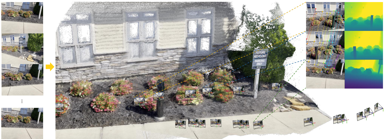
Figure 1. VGGT is a large feed-forward transformer with minimal 3D-inductive biases trained on a trove of 3D-annotated data. It accepts up to hundreds of images and predicts cameras, point maps, depth maps, and point tracks for all images at once in less than a second, which often outperforms optimization-based alternatives without further processing.
图 1: VGGT 是一个大型前馈 Transformer,具有最小的 3D 归纳偏差,并在大量 3D 标注数据上进行训练。它能够接受多达数百张图像,并在不到一秒的时间内一次性预测所有图像的相机、点图、深度图和点轨迹,通常优于基于优化的替代方案,且无需进一步处理。
Abstract
摘要
1. Introduction
1. 引言
We present VGGT, a feed-forward neural network that directly infers all key 3D attributes of a scene, including camera parameters, point maps, depth maps, and 3D point tracks, from one, a few, or hundreds of its views. This approach is a step forward in 3D computer vision, where models have typically been constrained to and specialized for single tasks. It is also simple and efficient, reconstructing images in under one second, and still outperforming alternatives that require post-processing with visual geometry optimization techniques. The network achieves state-of-the-art results in multiple 3D tasks, including camera parameter estimation, multi-view depth estimation, dense point cloud reconstruction, and 3D point tracking. We also show that using pretrained VGGT as a feature backbone significantly enhances downstream tasks, such as non-rigid point tracking and feed-forward novel view synthesis. Code and models are publicly available at https://github.com/facebook research/vggt.
我们提出了 VGGT,这是一种前馈神经网络,能够从一个、几个或数百个场景视图中直接推断出场景的所有关键 3D 属性,包括相机参数、点图、深度图和 3D 点轨迹。这种方法在 3D 计算机视觉领域迈出了一步,因为传统模型通常局限于单一任务并专门针对单一任务。VGGT 简单且高效,能够在一秒内重建图像,并且在不需要视觉几何优化技术后处理的情况下,仍然优于其他替代方案。该网络在多个 3D 任务中取得了最先进的结果,包括相机参数估计、多视图深度估计、密集点云重建和 3D 点跟踪。我们还展示了使用预训练的 VGGT 作为特征骨干可以显著增强下游任务,例如非刚性点跟踪和前馈新视图合成。代码和模型已在 https://github.com/facebookresearch/vggt 公开。
We consider the problem of estimating the 3D attributes of a scene, captured in a set of images, utilizing a feedforward neural network. Traditionally, 3D reconstruction has been approached with visual-geometry methods, utilizing iterative optimization techniques like Bundle Adjustment (BA) [45]. Machine learning has often played an important complementary role, addressing tasks that cannot be solved by geometry alone, such as feature matching and monocular depth prediction. The integration has become increasingly tight, and now state-of-the-art Structure-fromMotion (SfM) methods like VGGSfM [125] combine machine learning and visual geometry end-to-end via differentiable BA. Even so, visual geometry still plays a major role in 3D reconstruction, which increases complexity and computational cost.
我们考虑利用前馈神经网络从一组图像中估计场景的3D属性。传统上,3D重建通常通过视觉几何方法实现,使用诸如捆绑调整 (Bundle Adjustment, BA) [45] 的迭代优化技术。机器学习通常扮演重要的补充角色,解决仅靠几何无法完成的任务,例如特征匹配和单目深度预测。两者的结合越来越紧密,现在最先进的结构从运动 (Structure-from-Motion, SfM) 方法(如 VGGSfM [125])通过可微分的 BA 将机器学习和视觉几何端到端地结合起来。即便如此,视觉几何在3D重建中仍然占据重要地位,这增加了复杂性和计算成本。
As networks become ever more powerful, we ask if, finally, 3D tasks can be solved directly by a neural network, eschewing geometry post-processing almost entirely. Recent contributions like DUSt3R [129] and its evolution
随着网络变得越来越强大,我们不禁要问,是否最终可以通过神经网络直接解决3D任务,几乎完全避免几何后处理。最近的研究成果如DUSt3R [129] 及其演进
MASt3R [62] have shown promising results in this direction, but these networks can only process two images at once and rely on post-processing to reconstruct more images, fusing pairwise reconstructions.
MASt3R [62] 在这方面展示了有前景的结果,但这些网络一次只能处理两张图像,并依赖后处理来重建更多图像,融合成对重建。
In this paper, we take a further step towards removing the need to optimize 3D geometry in post-processing. We do so by introducing Visual Geometry Grounded Transformer (VGGT), a feed-forward neural network that performs 3D reconstruction from one, a few, or even hundreds of input views of a scene. VGGT predicts a full set of 3D attributes, including camera parameters, depth maps, point maps, and 3D point tracks. It does so in a single forward pass, in seconds. Remarkably, it often outperforms optimization-based alternatives even without further processing. This is a substantial departure from DUSt3R, MASt3R, or VGGSfM, which still require costly iterative post-optimization to obtain usable results.
在本文中,我们朝着消除后处理中对3D几何优化的需求迈出了进一步的一步。我们通过引入视觉几何基础Transformer (Visual Geometry Grounded Transformer, VGGT) 来实现这一目标,VGGT是一种前馈神经网络,能够从场景的一个、几个甚至数百个输入视图中执行3D重建。VGGT预测了一整套3D属性,包括相机参数、深度图、点图和3D点轨迹。它只需一次前向传递,耗时仅数秒。值得注意的是,即使不进行进一步处理,它通常也优于基于优化的替代方案。这与DUSt3R、MASt3R或VGGSfM有显著不同,这些方法仍然需要昂贵的迭代后优化才能获得可用的结果。
We also show that it is unnecessary to design a special network for 3D reconstruction. Instead, VGGT is based on a fairly standard large transformer [119], with no particular 3D or other inductive biases (except for alternating between frame-wise and global attention), but trained on a large number of publicly available datasets with 3D annotations. VGGT is thus built in the same mold as large models for natural language processing and computer vision, such as GPTs [1, 29, 148], CLIP [86], DINO [10, 78], and Stable Diffusion [34]. These have emerged as versatile backbones that can be fine-tuned to solve new, specific tasks. Similarly, we show that the features computed by VGGT can significantly enhance downstream tasks like point tracking in dynamic videos, and novel view synthesis.
我们还表明,没有必要为 3D 重建设计专门的网络。相反,VGGT 基于一个相当标准的大 Transformer [119],没有特定的 3D 或其他归纳偏差(除了在帧级注意力和全局注意力之间交替),但在大量带有 3D 标注的公开数据集上进行了训练。因此,VGGT 的构建方式与自然语言处理和计算机视觉领域的大模型(如 GPTs [1, 29, 148]、CLIP [86]、DINO [10, 78] 和 Stable Diffusion [34])相同。这些模型已经成为多功能骨干网络,可以通过微调来解决新的特定任务。同样,我们展示了 VGGT 计算的特征可以显著增强下游任务,如动态视频中的点跟踪和新视角合成。
There are several recent examples of large 3D neural networks, including Depth Anything [142], MoGe [128], and LRM [49]. However, these models only focus on a single 3D task, such as monocular depth estimation or novel view synthesis. In contrast, VGGT uses a shared backbone to predict all 3D quantities of interest together. We demonstrate that learning to predict these interrelated 3D attributes enhances overall accuracy despite potential redundancies. At the same time, we show that, during inference, we can derive the point maps from separately predicted depth and camera parameters, obtaining better accuracy compared to directly using the dedicated point map head.
最近有几个大型 3D 神经网络的例子,包括 Depth Anything [142]、MoGe [128] 和 LRM [49]。然而,这些模型只专注于单一的 3D 任务,例如单目深度估计或新视角合成。相比之下,VGGT 使用共享的主干网络来同时预测所有感兴趣的 3D 量。我们证明了尽管存在潜在的冗余,学习预测这些相互关联的 3D 属性可以提高整体准确性。同时,我们展示了在推理过程中,可以从单独预测的深度和相机参数中导出点云图,与直接使用专用的点云图头相比,可以获得更好的准确性。
To summarize, we make the following contributions: (1) We introduce VGGT, a large feed-forward transformer that, given one, a few, or even hundreds of images of a scene, can predict all its key 3D attributes, including camera intrinsics and extrinsics, point maps, depth maps, and 3D point tracks, in seconds. (2) We demonstrate that VGGT’s predictions are directly usable, being highly competitive and usually better than those of state-of-the-art methods that use slow post-processing optimization techniques. (3) We also show that, when further combined with BA post-processing,
总结来说,我们做出了以下贡献:(1) 我们提出了 VGGT,这是一个大型前馈 Transformer,给定一个场景的一张、几张甚至数百张图像,它可以在几秒钟内预测出所有关键的 3D 属性,包括相机内参和外参、点云图、深度图和 3D 点轨迹。(2) 我们证明了 VGGT 的预测结果可以直接使用,具有高度竞争力,并且通常优于使用缓慢后处理优化技术的最先进方法。(3) 我们还展示了,当进一步结合 BA 后处理时,
VGGT achieves state-of-the-art results across the board, even when compared to methods that specialize in a subset of 3D tasks, often improving quality substantially.
VGGT 在所有任务中都达到了最先进的成果,即使与专门针对 3D 任务子集的方法相比,也常常显著提高了质量。
We make our code and models publicly available at https://github.com/facebook research/vggt. We believe that this will facilitate further research in this direction and benefit the computer vision community by providing a new foundation for fast, reliable, and versatile 3D reconstruction.
我们在 https://github.com/facebook research/vggt 上公开了代码和模型。我们相信,这将为快速、可靠且多功能的 3D 重建提供新的基础,从而促进这一方向的进一步研究,并使计算机视觉社区受益。
2. Related Work
2. 相关工作
Structure from Motion is a classic computer vision problem [45, 77, 80] that involves estimating camera parameters and reconstructing sparse point clouds from a set of images of a static scene captured from different viewpoints. The traditional SfM pipeline [2, 36, 70, 94, 103, 134] consists of multiple stages, including image matching, triangulation, and bundle adjustment. COLMAP [94] is the most popular framework based on the traditional pipeline. In recent years, deep learning has improved many components of the SfM pipeline, with keypoint detection [21, 31, 116, 149] and image matching [11, 67, 92, 99] being two primary areas of focus. Recent methods [5, 102, 109, 112, 113, 118, 122, 125, 131, 160] explored end-to-end differentiable SfM, where VGGSfM [125] started to outperform traditional algorithms on challenging photo tourism scenarios.
运动结构恢复 (Structure from Motion, SfM) 是一个经典的计算机视觉问题 [45, 77, 80],它涉及从不同视角拍摄的一组静态场景图像中估计相机参数并重建稀疏点云。传统的 SfM 流程 [2, 36, 70, 94, 103, 134] 包括多个阶段,如图像匹配、三角测量和捆绑调整。COLMAP [94] 是基于传统流程的最流行框架。近年来,深度学习改进了 SfM 流程的许多组件,其中关键点检测 [21, 31, 116, 149] 和图像匹配 [11, 67, 92, 99] 是两个主要关注领域。最近的方法 [5, 102, 109, 112, 113, 118, 122, 125, 131, 160] 探索了端到端可微分的 SfM,其中 VGGSfM [125] 开始在具有挑战性的照片旅游场景中超越传统算法。
Multi-view Stereo aims to densely reconstruct the geometry of a scene from multiple overlapping images, typically assuming known camera parameters, which are often estimated with SfM. MVS methods can be divided into three categories: traditional handcrafted [38, 39, 96, 130], global optimization [37, 74, 133, 147], and learning-based methods [42, 72, 84, 145, 157]. As in SfM, learning-based MVS approaches have recently seen a lot of progress. Here, DUSt3R [129] and MASt3R [62] directly estimate aligned dense point clouds from a pair of views, similar to MVS but without requiring camera parameters. Some concurrent works [111, 127, 141, 156] explore replacing DUSt3R’s test-time optimization with neural networks, though these attempts achieve only suboptimal or comparable performance to DUSt3R. Instead, VGGT outperforms DUSt3R and MASt3R by a large margin.
多视图立体视觉 (Multi-view Stereo, MVS) 旨在从多个重叠图像中密集重建场景的几何结构,通常假设已知的相机参数,这些参数通常通过 SfM (Structure from Motion) 进行估计。MVS 方法可以分为三类:传统手工方法 [38, 39, 96, 130]、全局优化方法 [37, 74, 133, 147] 和基于学习的方法 [42, 72, 84, 145, 157]。与 SfM 类似,基于学习的 MVS 方法最近取得了很大进展。其中,DUSt3R [129] 和 MASt3R [62] 直接从一对视图中估计对齐的密集点云,类似于 MVS,但不需要相机参数。一些并行工作 [111, 127, 141, 156] 探索用神经网络替代 DUSt3R 的测试时优化,尽管这些尝试仅实现了次优或与 DUSt3R 相当的性能。相比之下,VGGT 大幅优于 DUSt3R 和 MASt3R。
Tracking-Any-Point was first introduced in Particle Video [91] and revived by PIPs [44] during the deep learning era, aiming to track points of interest across video sequences including dynamic motions. Given a video and some 2D query points, the task is to predict 2D correspondences of these points in all other frames. TAP-Vid [23] proposed three benchmarks for this task and a simple baseline method later improved in TAPIR [24]. CoTracker [55, 56] utilized correlations between different points to track through occlusions, while DOT [60] enabled dense tracking through occlusions. Recently, TAPTR [63] proposed an end-to-end transformer for this task, and LocoTrack [13] extended commonly used pointwise features to nearby regions. All of these methods are specialized point trackers. Here, we demonstrate that VGGT’s features yield state-ofthe-art tracking performance when coupled with existing point trackers.
Tracking-Any-Point 最初在 Particle Video [91] 中提出,并在深度学习时代由 PIPs [44] 重新引入,旨在跟踪视频序列中包括动态运动在内的兴趣点。给定一个视频和一些 2D 查询点,任务是在所有其他帧中预测这些点的 2D 对应关系。TAP-Vid [23] 为此任务提出了三个基准,并在 TAPIR [24] 中改进了简单的基线方法。CoTracker [55, 56] 利用不同点之间的相关性来跟踪遮挡,而 DOT [60] 则通过遮挡实现了密集跟踪。最近,TAPTR [63] 提出了一个端到端的 Transformer 来解决此任务,而 LocoTrack [13] 将常用的点特征扩展到附近区域。所有这些方法都是专门的点跟踪器。在这里,我们展示了 VGGT 的特征与现有点跟踪器结合时,能够实现最先进的跟踪性能。
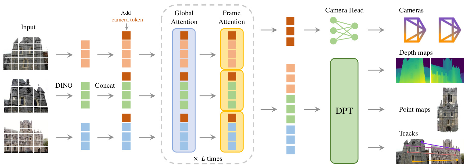
Figure 2. Architecture Overview. Our model first patchifies the input images into tokens by DINO, and appends camera tokens for camera prediction. It then alternates between frame-wise and global self attention layers. A camera head makes the final prediction for camera extrinsics and intrinsics, and a DPT [87] head for any dense output.
图 2: 架构概览。我们的模型首先通过 DINO 将输入图像分割为 Token,并附加相机 Token 用于相机预测。然后,它在帧级和全局自注意力层之间交替。相机头负责最终预测相机外参和内参,而 DPT [87] 头则负责任何密集输出。
3. Method
3. 方法
We introduce VGGT, a large transformer that ingests a set of images as input and produces a variety of 3D quantities as output. We start by introducing the problem in Sec. 3.1, followed by our architecture in Sec. 3.2 and its prediction heads in Sec. 3.3, and finally the training setup in Sec. 3.4.
我们介绍了 VGGT,这是一个大型 Transformer,它接收一组图像作为输入,并生成多种 3D 量作为输出。我们首先在第 3.1 节中介绍了问题,然后在第 3.2 节中介绍了我们的架构,接着在第 3.3 节中介绍了其预测头,最后在第 3.4 节中介绍了训练设置。
3.1. Problem definition and notation
3.1. 问题定义与符号表示
The input is a sequence $(I_{i}){i=1}^{N}$ of $N$ RGB images $I{i}\in\mathbf{\Gamma}$ R3×H×W , observing the same 3D scene. VGGT’s transformer is a function that maps this sequence to a corresponding set of 3D annotations, one per frame:
输入是一个由 $N$ 个 RGB 图像组成的序列 $(I_{i}){i=1}^{N}$,其中 $I{i}\in\mathbf{\Gamma}$ R3×H×W,观察的是同一个 3D 场景。VGGT 的 Transformer 是一个函数,将这个序列映射到一组对应的 3D 标注,每帧一个:

The transformer thus maps each image $I_{i}$ to its camera parameters $\mathbf{g}{i}\in\mathbb{R}^{9}$ (intrinsics and extrinsics), its depth map $D{i}\in\mathbb{R}^{H\times W}$ , its point map $P_{i}\in\mathbb{R}^{3\times H\times W}$ , and a grid $T_{i}\in\mathbb{R}^{C\times H\times W}$ of $C$ -dimensional features for point tracking. We explain next how these are defined.
Transformer 因此将每个图像 $I_{i}$ 映射到其相机参数 $\mathbf{g}{i}\in\mathbb{R}^{9}$(内参和外参)、深度图 $D{i}\in\mathbb{R}^{H\times W}$、点图 $P_{i}\in\mathbb{R}^{3\times H\times W}$,以及用于点跟踪的 $C$ 维特征网格 $T_{i}\in\mathbb{R}^{C\times H\times W}$。接下来我们将解释这些内容的定义。
For the camera parameters $\mathbf{g}{i}$ , we use the para me tri zation from [125] and set $\mathbf{g}=[\mathbf{q},\mathbf{t},\mathbf{f}]$ which is the concatenation of the rotation quaternion $\mathbf{q}\in\mathbb{R}^{4}$ , the translation vec- tor $\mathbf{t}\in\mathbb{R}^{3}$ , and the field of view $\mathbf{f{\alpha}}\in\mathbb{R}^{2}$ . We assume that the camera’s principal point is at the image center, which is common in SfM frameworks [95, 125].
对于相机参数 $\mathbf{g}{i}$,我们使用 [125] 中的参数化方法,并设置 $\mathbf{g}=[\mathbf{q},\mathbf{t},\mathbf{f}]$,这是旋转四元数 $\mathbf{q}\in\mathbb{R}^{4}$、平移向量 $\mathbf{t}\in\mathbb{R}^{3}$ 和视场角 $\mathbf{f{\alpha}}\in\mathbb{R}^{2}$ 的拼接。我们假设相机的主点位于图像中心,这在 SfM 框架中很常见 [95, 125]。
We denote the domain of the image $I_{i}$ with $\begin{array}{r l}{\mathbb{}Z(I_{i})}&{{}=}\end{array}$ ${1,\dots,H}\times{1,\dots,W}$ , i.e., the set of pixel locations. The depth map $D_{i}$ associates each pixel location $\mathbf{y}\in\mathcal{I}(I_{i})$ with its corresponding depth value $D_{i}(\mathbf{y})\in\mathbb{R}^{+}$ , as observed from the $i$ -th camera. Likewise, the point map $P_{i}$ associates each pixel with its corresponding 3D scene point $P_{i}(\mathbf{y})\in\mathbb{R}^{3}$ . Importantly, like in DUSt3R [129], the point maps are viewpoint invariant, meaning that the 3D points $P_{i}(\mathbf{y})$ are defined in the coordinate system of the first camera ${\bf g}_{1}$ , which we take as the world reference frame.
我们将图像 $I_{i}$ 的域表示为 $\begin{array}{r l}{\mathbb{}Z(I_{i})}&{{}=}\end{array}$ ${1,\dots,H}\times{1,\dots,W}$,即像素位置的集合。深度图 $D_{i}$ 将每个像素位置 $\mathbf{y}\in\mathcal{I}(I_{i})$ 与其对应的深度值 $D_{i}(\mathbf{y})\in\mathbb{R}^{+}$ 关联起来,这是从第 $i$ 个相机观察到的。同样,点图 $P_{i}$ 将每个像素与其对应的 3D 场景点 $P_{i}(\mathbf{y})\in\mathbb{R}^{3}$ 关联起来。重要的是,与 DUSt3R [129] 中一样,点图是视角不变的,这意味着 3D 点 $P_{i}(\mathbf{y})$ 是在第一个相机 ${\bf g}_{1}$ 的坐标系中定义的,我们将其作为世界参考系。
Finally, for keypoint tracking, we follow track-anypoint methods such as [25, 57]. Namely, given a fixed query image point ${\bf y}{q}$ in the query image $I{q}$ , the network outputs a track $\begin{array}{r}{\mathcal{T}^{\star}(\mathbf{y}{q})^{\star}=(\mathbf{y}{i}){i=1}^{N}}\end{array}$ formed by the corresponding 2D points $\mathbf{y}{i}\in\mathbb{R}^{2}$ in all images $I_{i}$ .
最后,对于关键点跟踪,我们遵循诸如 [25, 57] 的 track-anypoint 方法。即,给定查询图像 $I_{q}$ 中的一个固定查询图像点 ${\bf y}{q}$,网络输出一个由所有图像 $I{i}$ 中的对应 2D 点 $\mathbf{y}{i}\in\mathbb{R}^{2}$ 组成的轨迹 $\begin{array}{r}{\mathcal{T}^{\star}(\mathbf{y}{q})^{\star}=(\mathbf{y}{i}){i=1}^{N}}\end{array}$。
Note that the transformer $f$ above does not output the tracks directly but instead features $\boldsymbol{T_{i}}\in\mathbb{R}^{C\times H\times W}$ , which are used for tracking. The tracking is delegated to a separate module, described in Sec. 3.3, which implements a function $\mathcal{T}((\mathbf{y}{j}){j=1}^{M},(T_{i})_{i=1}^{N})=((\hat{\mathbf{y}}_{j,i})_{i=1}^{N})_{j=1}^{M}$ . It ingests the query point ${\bf y}_{q}$ and the dense tracking features $T_{i}$ output by the transformer $f$ and then computes the track. The two networks $f$ and $\tau$ are trained jointly end-to-end.
注意,上述的 Transformer $f$ 并不直接输出轨迹,而是输出用于跟踪的特征 $\boldsymbol{T_{i}}\in\mathbb{R}^{C\times H\times W}$。跟踪任务被委托给一个单独的模块,该模块在 3.3 节中描述,它实现了一个函数 $\mathcal{T}((\mathbf{y}{j}){j=1}^{M},(T_{i})_{i=1}^{N})=((\hat{\mathbf{y}}_{j,i})_{i=1}^{N})_{j=1}^{M}$。该模块接收查询点 ${\bf y}_{q}$ 和由 Transformer $f$ 输出的密集跟踪特征 $T_{i}$,然后计算轨迹。两个网络 $f$ 和 $\tau$ 是端到端联合训练的。
Order of Predictions. The order of the images in the input sequence is arbitrary, except that the first image is chosen as the reference frame. The network architecture is designed to be permutation e qui variant for all but the first frame.
预测顺序。输入序列中图像的顺序是任意的,除了第一张图像被选为参考帧。网络架构设计为对除第一帧外的所有帧具有排列等变性。
Over-complete Predictions. Notably, not all quantities predicted by VGGT are independent. For example, as shown by DUSt3R [129], the camera parameters $\mathbf{g}$ can be inferred from the invariant point map $P$ , for instance, by solving the Perspective $^{\cdot n}$ -Point $(\mathrm{{PnP})}$ problem [35, 61].
过度完整的预测。值得注意的是,VGGT 预测的所有量并不都是独立的。例如,如 DUSt3R [129] 所示,相机参数 $\mathbf{g}$ 可以从不变点图 $P$ 中推断出来,例如通过解决 Perspective $^{\cdot n}$ -Point $(\mathrm{{PnP})}$ 问题 [35, 61]。
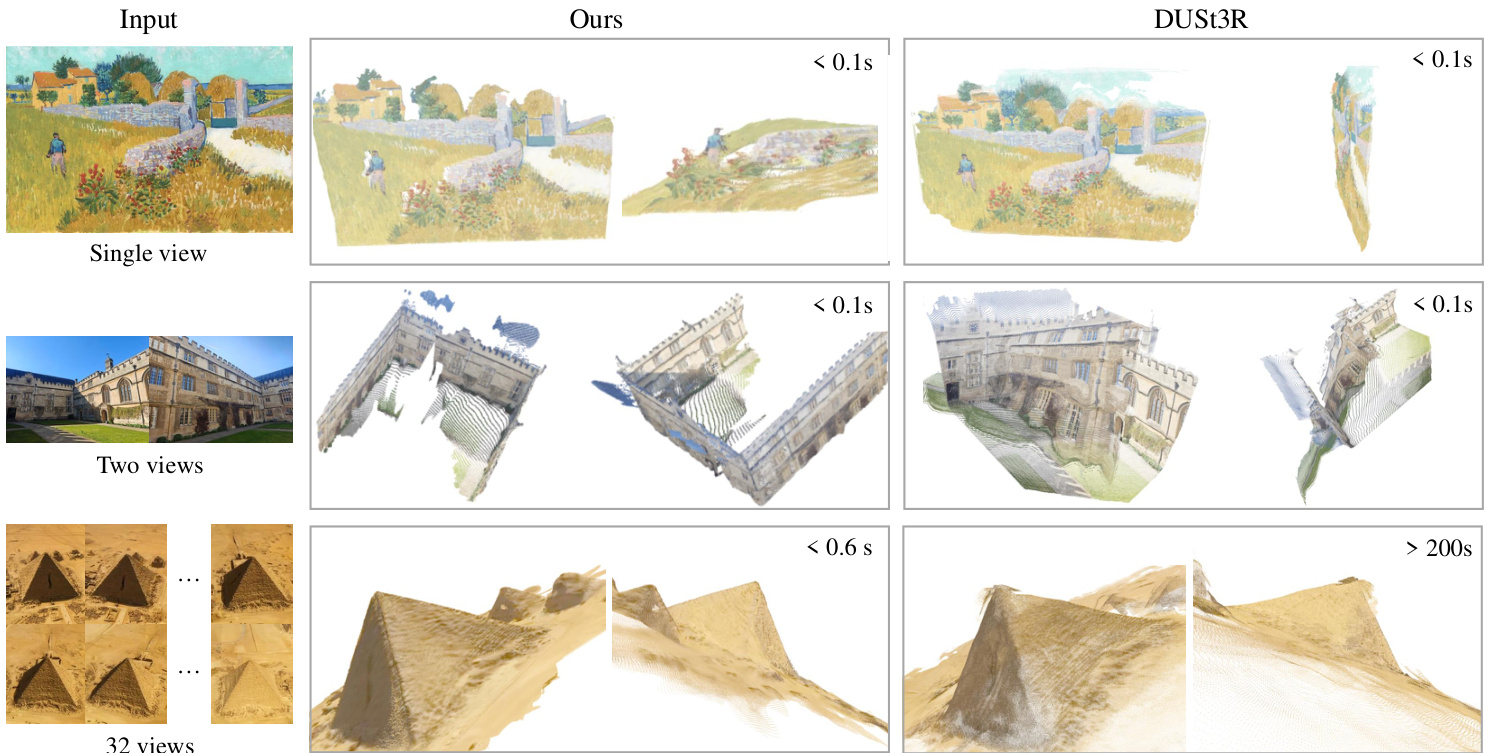
Figure 3. Qualitative comparison of our predicted 3D points to DUSt3R on in-the-wild images. As shown in the top row, our method successfully predicts the geometric structure of an oil painting, while DUSt3R predicts a slightly distorted plane. In the second row, our method correctly recovers a 3D scene from two images with no overlap, while DUSt3R fails. The third row provides a challenging example with repeated textures, while our prediction is still high-quality. We do not include examples with more than 32 frames, as DUSt3R runs out of memory beyond this limit.
图 3: 我们的预测 3D 点与 DUSt3R 在野外图像上的定性对比。如第一行所示,我们的方法成功预测了一幅油画的几何结构,而 DUSt3R 预测了一个略微扭曲的平面。在第二行中,我们的方法从两张没有重叠的图像中正确恢复了 3D 场景,而 DUSt3R 失败了。第三行提供了一个具有重复纹理的挑战性示例,而我们的预测仍然是高质量的。我们没有包含超过 32 帧的示例,因为 DUSt3R 在此限制之外会耗尽内存。
Furthermore, the depth maps can be deduced from the point map and the camera parameters. However, as we show in Sec. 4.5, tasking VGGT with explicitly predicting all aforementioned quantities during training brings substantial performance gains, even when these are related by closed-form relationships. Meanwhile, during inference, it is observed that combining independently estimated depth maps and camera parameters produces more accurate 3D points compared to directly employing a specialized point map branch.
此外,深度图可以从点云图和相机参数中推导出来。然而,正如我们在第4.5节中所示,在训练过程中让VGGT显式预测所有上述量会带来显著的性能提升,即使这些量之间存在闭式关系。同时,在推理过程中,观察到结合独立估计的深度图和相机参数比直接使用专门的点云图分支能产生更准确的3D点。
3.2. Feature Backbone
3.2. 特征骨干网络
Following recent works in 3D deep learning [53, 129, 132], we design a simple architecture with minimal 3D inductive biases, letting the model learn from ample quantities of 3D-annotated data. In particular, we implement the model $f$ as a large transformer [119]. To this end, each input image $I$ is initially patchified into a set of $K$ tokens1 $\mathrm{t}^{I}\in\mathbb{R}^{K\times C}$ through DINO [78]. The combined set of image tokens from all frames, i.e., $\mathrm{t}^{I}=\cup_{i=1}^{N}{\mathrm{t}_{i}^{I}}$ , is subsequently processed through the main network structure, alternating frame-wise and global self-attention layers.
遵循近期3D深度学习的研究 [53, 129, 132],我们设计了一个具有最小3D归纳偏置的简单架构,让模型从大量的3D标注数据中学习。具体来说,我们将模型 $f$ 实现为一个大型Transformer [119]。为此,每个输入图像 $I$ 首先通过DINO [78] 被分割成一组 $K$ 个Token $\mathrm{t}^{I}\in\mathbb{R}^{K\times C}$。所有帧的图像Token组合,即 $\mathrm{t}^{I}=\cup_{i=1}^{N}{\mathrm{t}_{i}^{I}}$,随后通过主网络结构进行处理,交替使用帧内和全局自注意力层。
Alternating-Attention. We slightly adjust the standard transformer design by introducing Alternating-Attention (AA), making the transformer focus within each frame and globally in an alternate fashion. Specifically, frame-wise self-attention attends to the tokens $\mathrm{t}_{k}^{I}$ within each frame separately, and global self-attention attends to the tokens $\mathrm{t}^{I}$ across all frames jointly. This strikes a balance between integrating information across different images and normalizing the activation s for the tokens within each image. By default, we employ $L=24$ layers of global and frame-wise attention. In Sec. 4, we demonstrate that our AA architecture brings significant performance gains. Note that our architecture does not employ any cross-attention layers, only self-attention ones.
交替注意力 (Alternating-Attention)。我们通过引入交替注意力 (AA) 对标准 Transformer 设计进行了轻微调整,使 Transformer 以交替方式在每帧内和全局范围内聚焦。具体来说,帧内自注意力 (frame-wise self-attention) 分别关注每帧内的 Token $\mathrm{t}_{k}^{I}$,而全局自注意力 (global self-attention) 则联合关注所有帧中的 Token $\mathrm{t}^{I}$。这在整合不同图像之间的信息和归一化每张图像内 Token 的激活之间取得了平衡。默认情况下,我们使用 $L=24$ 层全局和帧内注意力。在第 4 节中,我们展示了我们的 AA 架构带来了显著的性能提升。请注意,我们的架构没有使用任何交叉注意力层,仅使用了自注意力层。
3.3. Prediction heads
3.3 预测头
Here, we describe how $f$ predicts the camera parameters, depth maps, point maps, and point tracks. First, for each input image $I_{i}$ , we augment the corresponding image tokens $\mathrm{t}{i}^{I}$ with an additional camera token $\mathbf{t}{i}^{\mathbf{g}}\in\mathbf{\mathbb{R}}^{1\times\check{C^{\prime}}}$ and four register tokens [19] $\mathbf{t}{i}^{R}\in\mathbb{R}^{4\times C^{\prime}}$ . The concatenation of $(\mathbf{t}{i}^{I},\mathbf{t}{i}^{\mathbf{g}},\mathbf{t}{i}^{R}j){i=1}^{N}$ is then passed to the AA transformer, yieldingoutput ensecamek and register tokens of the first frame $(\mathrm{t}{1}^{\mathbf{g}}:=\bar{\mathrm{t}}^{\mathbf{g}}$ , $\mathrm{t}_{1}^{R}:=\bar{\mathrm{t}}^{R})$ are set to a different set of learnable tokens $\bar{\mathrm{t}}^{\mathbf{g}},\bar{\mathrm{t}}^{R}$ than those of all other frames $(\mathbf{t}_{i}^{\mathbf{g}}:=\bar{\mathbf{t}}^{\mathbf{g}},\mathbf{t}_{i}^{R}:=\bar{\mathbf{t}}^{R},i\in[2,\dots,N])$ , which are also learnable. This allows the model to distinguish the first frame from the rest, and to represent the 3D predictions in the coordinate frame of the first camera. Note that the refined camera and register tokens now become frame-specific—–this is because our AA transformer contains frame-wise self-attention layers that allow the transformer to match the camera and register tokens with the corresponding tokens from the same image. Following common practice, the output register tokens $\hat{\mathbf{t}}_{i}^{R}$ are discarded while $\hat{\bf t}_{i}^{I},\hat{\bf t}_{i}^{\bf g}$ are used for prediction.
在这里,我们描述了 $f$ 如何预测相机参数、深度图、点云图和点轨迹。首先,对于每个输入图像 $I_{i}$,我们用额外的相机 token $\mathbf{t}{i}^{\mathbf{g}}\in\mathbf{\mathbb{R}}^{1\times\check{C^{\prime}}}$ 和四个寄存器 token [19] $\mathbf{t}{i}^{R}\in\mathbb{R}^{4\times C^{\prime}}$ 来增强相应的图像 token $\mathrm{t}{i}^{I}$。然后将 $(\mathbf{t}{i}^{I},\mathbf{t}{i}^{\mathbf{g}},\mathbf{t}{i}^{R}j){i=1}^{N}$ 的连接传递给 AA Transformer,生成输出。第一帧的相机 token 和寄存器 token $(\mathrm{t}{1}^{\mathbf{g}}:=\bar{\mathrm{t}}^{\mathbf{g}}$,$\mathrm{t}_{1}^{R}:=\bar{\mathrm{t}}^{R})$ 被设置为与所有其他帧 $(\mathbf{t}_{i}^{\mathbf{g}}:=\bar{\mathbf{t}}^{\mathbf{g}},\mathbf{t}_{i}^{R}:=\bar{\mathbf{t}}^{R},i\in[2,\dots,N])$ 不同的可学习 token $\bar{\mathrm{t}}^{\mathbf{g}},\bar{\mathrm{t}}^{R}$,这些 token 也是可学习的。这使得模型能够区分第一帧与其他帧,并在第一帧相机的坐标系中表示 3D 预测。请注意,优化后的相机 token 和寄存器 token 现在变得特定于帧——这是因为我们的 AA Transformer 包含帧级自注意力层,允许 Transformer 将相机 token 和寄存器 token 与来自同一图像的相应 token 进行匹配。按照常规做法,输出寄存器 token $\hat{\mathbf{t}}_{i}^{R}$ 被丢弃,而 $\hat{\bf t}_{i}^{I},\hat{\bf t}_{i}^{\bf g}$ 用于预测。
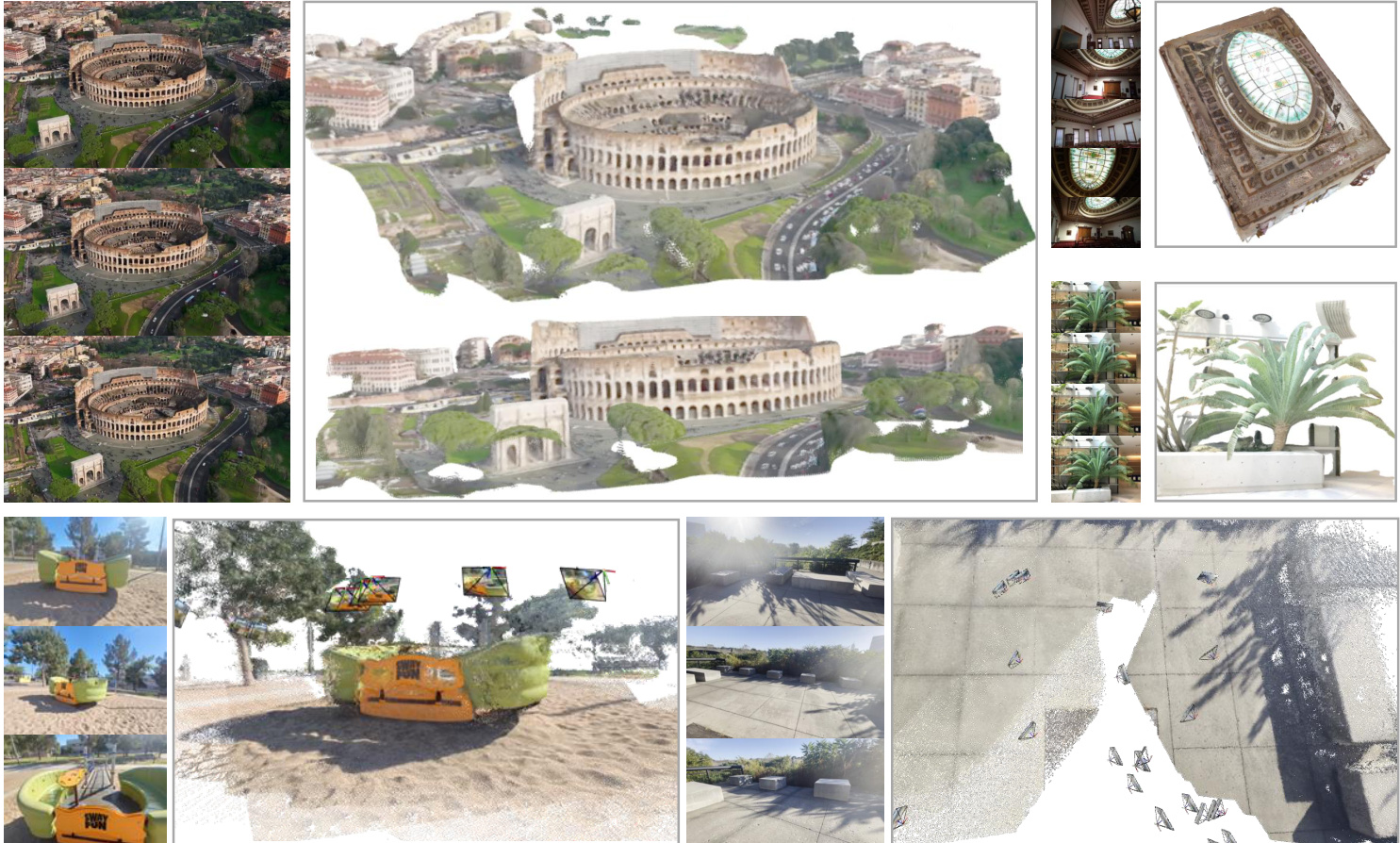
Figure 4. Additional Visualization s of Point Map Estimation. Camera frustums illustrate the estimated camera poses. Explore our interactive demo for better visualization quality.
图 4: 点云地图估计的附加可视化。相机视锥体展示了估计的相机姿态。请访问我们的交互式演示以获得更好的可视化效果。
Coordinate Frame. As noted above, we predict cameras, point maps, and depth maps in the coordinate frame of the first camera ${\bf g}{1}$ . As such, the camera extrinsics output for the first camera are set to the identity, i.e., the first rotation quaternion is $\mathbf{q}{1}=[0,0,0,1]$ and the first translation vector is $\mathbf{t}_{1}=[0,0,0]$ . Recall that the special camera and register tokens $\mathbf{t}_{1}^{\mathbf{g}}:=\overline{{\mathbf{t}}}^{\mathbf{g}},\mathbf{t}_{1}^{R}:=\overline{{\mathbf{t}}}^{R}$ allow the transformer to identify the first camera.
坐标系。如上所述,我们在第一个相机 ${\bf g}{1}$ 的坐标系中预测相机、点云图和深度图。因此,第一个相机的外参输出被设置为单位矩阵,即第一个旋转四元数为 $\mathbf{q}{1}=[0,0,0,1]$,第一个平移向量为 $\mathbf{t}_{1}=[0,0,0]$。需要注意的是,特殊的相机和注册 token $\mathbf{t}_{1}^{\mathbf{g}}:=\overline{{\mathbf{t}}}^{\mathbf{g}},\mathbf{t}_{1}^{R}:=\overline{{\mathbf{t}}}^{R}$ 允许 Transformer 识别第一个相机。
Camera Predictions. The camera parameters $(\hat{\mathbf{g}}^{i}){i=1}^{N}$ are predicted from the output camera tokens $(\hat{\mathrm{t}}{i}^{\mathbf{g}})_{i=1}^{N}$ using four additional self-attention layers followed by a linear layer. This forms the camera head that predicts the camera intrin
相机预测。相机参数 $(\hat{\mathbf{g}}^{i}){i=1}^{N}$ 通过四个额外的自注意力层和一个线性层从输出的相机 token $(\hat{\mathrm{t}}{i}^{\mathbf{g}})_{i=1}^{N}$ 中预测得出。这构成了预测相机内参的相机头。
sics and extrinsics.
sics 和 extrinsics。
Dense Predictions. The output image tokens $\hat{\mathrm{t}}{i}^{I}$ are used to predict the dense outputs, $i.e.$ ., the depth maps $D{i}$ , point maps $P_{i}$ , and tracking features $T_{i}$ . More specifically, $\hat{\mathrm{t}}{i}^{I}$ are first converted to dense feature maps $F{i}\in\mathbb{R}^{C^{\prime\prime}\times H\times W}$ with a DPT layer [87]. Each $F_{i}$ is then mapped with a $3\times3$ convolutional layer to the corresponding depth and point maps $D_{i}$ and $P_{i}$ . Additionally, the DPT head also outputs dense features $T_{i}\in\mathbb{R}^{C\times H\times\dot{W}}$ , which serve as input to the tracking head. We also predict the aleatoric uncertainty [58, 76] $\Sigma_{i}^{\breve{D}}\in\mathbb{R}{+}^{H\times W}$ and $\Sigma{i}^{P}\in\mathbb{R}_{+}^{H\times W}$ for each depth and point map, respectively. As described in Sec. 3.4, the uncertainty maps are used in the loss and, after training, are proportional to the model’s confidence in the predictions.
密集预测。输出图像 token $\hat{\mathrm{t}}{i}^{I}$ 用于预测密集输出,即深度图 $D{i}$、点图 $P_{i}$ 和跟踪特征 $T_{i}$。具体来说,$\hat{\mathrm{t}}{i}^{I}$ 首先通过 DPT 层 [87] 转换为密集特征图 $F{i}\in\mathbb{R}^{C^{\prime\prime}\times H\times W}$。然后,每个 $F_{i}$ 通过一个 $3\times3$ 卷积层映射到相应的深度图和点图 $D_{i}$ 和 $P_{i}$。此外,DPT 头还输出密集特征 $T_{i}\in\mathbb{R}^{C\times H\times\dot{W}}$,作为跟踪头的输入。我们还分别预测了每个深度图和点图的随机不确定性 [58, 76] $\Sigma_{i}^{\breve{D}}\in\mathbb{R}{+}^{H\times W}$ 和 $\Sigma{i}^{P}\in\mathbb{R}_{+}^{H\times W}$。如第 3.4 节所述,不确定性图用于损失计算,并且在训练后与模型对预测的置信度成正比。
Tracking. In order to implement the tracking module $\tau$ , we use the CoTracker2 architecture [57], which takes the dense tracking features $T_{i}$ as input. More specifically, given a query point $\mathbf{y}{j}$ in a query image $I{q}$ (during training, we always set $q=1$ , but any other image can be potentially used as a query), the tracking head $\tau$ predicts the set of 2D points $\mathcal{T}((\mathbf{y}{j}){j=1}^{M},(T_{i})_{i=1}^{N})=((\hat{\mathbf{y}}_{j,i})_{i=1}^{N})_{j=1}^{M}$ in all images $I_{i}$ that correspond to the same 3D point as $\mathbf{y}$ . To do so, the feature map $T_{q}$ of the query image is first bilinearly sampled at the query point $\mathbf{y}_{j}$ to obtain its feature. This feature is then correlated with all other feature maps $T_{i},i\neq q$ to obtain a set of correlation maps. These maps are then processed by self-attention layers to predict the final 2D points $\hat{\mathbf{y}}_{i}$ , which are all in correspondence with $\mathbf{y}_{j}$ . Note that, similar to VGGSfM [125], our tracker does not assume any temporal ordering of the input frames and, hence, can be applied to any set of input images, not just videos.
为了实现跟踪模块 $\tau$,我们使用了 CoTracker2 架构 [57],该架构以密集跟踪特征 $T_{i}$ 作为输入。具体来说,给定查询图像 $I_{q}$ 中的查询点 $\mathbf{y}{j}$(在训练过程中,我们始终设置 $q=1$,但任何其他图像也可以作为查询图像),跟踪头 $\tau$ 预测在所有图像 $I{i}$ 中与 $\mathbf{y}$ 对应的 3D 点相同的 2D 点集 $\mathcal{T}((\mathbf{y}{j}){j=1}^{M},(T_{i})_{i=1}^{N})=((\hat{\mathbf{y}}_{j,i})_{i=1}^{N})_{j=1}^{M}$。为此,首先在查询点 $\mathbf{y}_{j}$ 处对查询图像的特征图 $T_{q}$ 进行双线性采样,以获取其特征。然后将该特征与所有其他特征图 $T_{i},i\neq q$ 进行相关,得到一组相关图。这些相关图随后通过自注意力层处理,以预测最终的 2D 点 $\hat{\mathbf{y}}_{i}$,这些点都与 $\mathbf{y}_{j}$ 对应。需要注意的是,与 VGGSfM [125] 类似,我们的跟踪器不假设输入帧的任何时间顺序,因此可以应用于任何输入图像集,而不仅仅是视频。
3.4. Training
3.4. 训练
Training Losses. We train the VGGT model $f$ end-to-end using a multi-task loss:
训练损失。我们使用多任务损失端到端地训练 VGGT 模型 $f$:
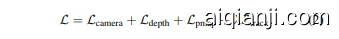
We found that the camera $(\mathcal{L}{\mathrm{camera}})$ , depth $(\mathcal{L}{\mathrm{depth}})$ , and point-map $(\mathcal{L}{\mathrm{pmap}})$ losses have similar ranges and do not need to be weighted against each other. The tracking loss $\mathcal{L}{\mathrm{track}}$ is down-weighted with a factor of $\lambda=0.05$ . We describe each loss term in turn.
我们发现相机损失 $(\mathcal{L}{\mathrm{camera}})$ 、深度损失 $(\mathcal{L}{\mathrm{depth}})$ 和点图损失 $(\mathcal{L}{\mathrm{pmap}})$ 的范围相似,不需要相互加权。跟踪损失 $\mathcal{L}{\mathrm{track}}$ 被下调权重,因子为 $\lambda=0.05$。我们依次描述每个损失项。
The camera loss $\mathcal{L}{\mathrm{camera}}$ supervises the cameras $\hat{\bf g}$ $\begin{array}{r}{\mathcal{L}{\mathrm{camera}}=\sum_{i=1}^{N}\Vert\hat{\mathbf{g}}_{i}-\mathbf{g}_{i}\Vert_{\epsilon}}\end{array}$ , comparing the predicted cameras $\hat{\bf g}_{i}$ wi th the ground truth $\mathbf{g}_{i}$ using the Huber loss $|\cdot|_{\epsilon}$ .
相机损失 $\mathcal{L}{\mathrm{camera}}$ 监督相机 $\hat{\bf g}$ $\begin{array}{r}{\mathcal{L}{\mathrm{camera}}=\sum_{i=1}^{N}\Vert\hat{\mathbf{g}}_{i}-\mathbf{g}_{i}\Vert_{\epsilon}}\end{array}$,通过使用 Huber 损失 $|\cdot|_{\epsilon}$ 将预测的相机 $\hat{\bf g}_{i}$ 与真实值 $\mathbf{g}_{i}$ 进行比较。
The depth loss $\mathcal{L}{\mathrm{depth}}$ follows DUSt3R [129] and implements the aleatoric-uncertainty loss [59, 75] weighing the discrepancy between the predicted depth $\hat{D}{i}$ and the ground-truth depth $D_{i}$ with the predicted uncertainty map $\bar{\hat{\Sigma}}{i}^{D}$ . Differently from DUSt3R, we also apply a gradientbased term, which is widely used in monocular depth estimation. Hence, the depth loss is $\begin{array}{r}{\mathcal{L}{\mathrm{depth}}=\sum_{i=1}^{N}\dot{|}\Sigma_{i}^{D}\odot}\end{array}$ $(\hat{D}_{i}-D_{i})|+|\Sigma_{i}^{D}\odot(\nabla\hat{D}_{i}-\nabla D_{i})|\overset{\cdot}{-}\alpha\log{\Sigma_{i}^{D}}$ , where $\odot$ is the channel-broadcast element-wise product. The point map loss is defined analogously but with the point-map uncertainty $\begin{array}{r}{\Sigma_{i}^{P}\colon\mathcal{L}_{\mathrm{pmap}}=\sum_{i=1}^{N}|\Sigma_{i}^{P}\odot(\hat{P}_{i}-\dot{P}_{i})|+|\dot{\Sigma}_{i}^{P}\odot}\end{array}$ $(\nabla\hat{P}_{i}-\nabla P_{i})|-\alpha\log{\Sigma_{i}^{P}}$ .
深度损失 $\mathcal{L}{\mathrm{depth}}$ 遵循 DUSt3R [129],并实现了基于不确定性的损失 [59, 75],通过预测的不确定性图 $\bar{\hat{\Sigma}}{i}^{D}$ 来加权预测深度 $\hat{D}{i}$ 与真实深度 $D{i}$ 之间的差异。与 DUSt3R 不同的是,我们还应用了基于梯度的项,这在单目深度估计中被广泛使用。因此,深度损失为 $\begin{array}{r}{\mathcal{L}{\mathrm{depth}}=\sum{i=1}^{N}\dot{|}\Sigma_{i}^{D}\odot}\end{array}$ $(\hat{D}{i}-D{i})|+|\Sigma_{i}^{D}\odot(\nabla\hat{D}{i}-\nabla D{i})|\overset{\cdot}{-}\alpha\log{\Sigma_{i}^{D}}$ ,其中 $\odot$ 是通道广播的逐元素乘积。点图损失的定义类似,但使用点图不确定性 $\begin{array}{r}{\Sigma_{i}^{P}\colon\mathcal{L}_{\mathrm{pmap}}=\sum_{i=1}^{N}|\Sigma_{i}^{P}\odot(\hat{P}_{i}-\dot{P}_{i})|+|\dot{\Sigma}_{i}^{P}\odot}\end{array}$ $(\nabla\hat{P}_{i}-\nabla P_{i})|-\alpha\log{\Sigma_{i}^{P}}$ 。
Finally, the tracking loss is given by $\begin{array}{r l}{\mathcal{L}{\mathrm{track}}}&{{}=}\end{array}$ $\begin{array}{r}{\sum{j=1}^{M}\sum_{i=1}^{N}|\mathbf{y}_{j,i}-\hat{\mathbf{y}}_{j,i}|}\end{array}$ . Here, the outer sum runs over all ground-truth query points $\mathbf{y}_{j}$ in the query image $I_{q}$ , $\mathbf{y}_{j,i}$ is $\mathbf{y}_{j}$ ’s ground-truth correspondence in image $I_{i}$ , and $\hat{\mathbf{y}}_{j,i}$ is the corresponding prediction obtained by the application $\mathcal{T}((\mathbf{y}_{j})_{j=1}^{M},\mathbf{\bar{(}}T_{i})_{i=1}^{N}\mathbf{\bar{)}}$ of the tracking module. Additionally, following CoTracker2 [57], we apply a visibility loss (binary cross-entropy) to estimate whether a point is visible in a given frame.
最后,跟踪损失由 $\begin{array}{r l}{\mathcal{L}{\mathrm{track}}}&{{}=}\end{array}$ $\begin{array}{r}{\sum{j=1}^{M}\sum_{i=1}^{N}|\mathbf{y}_{j,i}-\hat{\mathbf{y}}_{j,i}|}\end{array}$ 给出。这里,外部的求和遍历查询图像 $I_{q}$ 中的所有真实查询点 $\mathbf{y}_{j}$,$\mathbf{y}_{j,i}$ 是 $\mathbf{y}_{j}$ 在图像 $I_{i}$ 中的真实对应点,而 $\hat{\mathbf{y}}_{j,i}$ 是通过跟踪模块的应用 $\mathcal{T}((\mathbf{y}_{j})_{j=1}^{M},\mathbf{\bar{(}}T_{i})_{i=1}^{N}\mathbf{\bar{)}}$ 获得的相应预测。此外,遵循 CoTracker2 [57],我们应用可见性损失(二元交叉熵)来估计一个点是否在给定帧中可见。
Ground Truth Coordinate Normalization. If we scale a scene or change its global reference frame, the images of the scene are not affected at all, meaning that any such variant is a legitimate result of 3D reconstruction. We remove this ambiguity by normalizing the data, thus making a canonical choice and task the transformer to output this particular variant. We follow [129] and, first, express all quantities in the coordinate frame of the first camera ${\bf g}_{1}$ . Then, we compute the average Euclidean distance of all 3D points in the point map $P$ to the origin and use this scale to normalize the camera translations $\mathbf{t}$ , the point map $P$ , and the depth map $D$ . Importantly, unlike [129], we do not apply such normalization to the predictions output by the transformer; instead, we force it to learn the normalization we choose from the training data.
真实坐标归一化。如果我们缩放场景或改变其全局参考系,场景的图像不会受到任何影响,这意味着任何此类变体都是3D重建的合法结果。我们通过归一化数据来消除这种歧义,从而做出规范选择,并让Transformer输出这种特定变体。我们遵循[129],首先将所有量表示在第一个相机${\bf g}_{1}$的坐标系中。然后,我们计算点图$P$中所有3D点到原点的平均欧几里得距离,并使用此比例对相机平移$\mathbf{t}$、点图$P$和深度图$D$进行归一化。重要的是,与[129]不同,我们不将这种归一化应用于Transformer输出的预测;相反,我们强制它从训练数据中学习我们选择的归一化。
Implementation Details. By default, we employ $L=24$ layers of global and frame-wise attention, respectively. The model consists of approximately 1.2 billion parameters in total. We train the model by optimizing the training loss (2) with the AdamW optimizer for 160K iterations. We use a cosine learning rate scheduler with a peak learning rate of 0.0002 and a warmup of 8K iterations. For every batch, we randomly sample 2–24 frames from a random training scene. The input frames, depth maps, and point maps are resized to a maximum dimension of 518 pixels. The aspect ratio is randomized between 0.33 and 1.0. We also randomly apply color jittering, Gaussian blur, and grayscale augmentation to the frames. The training runs on 64 A100 GPUs over nine days. We employ gradient norm clipping with a threshold of 1.0 to ensure training stability. We leverage bfloat16 precision and gradient check pointing to improve GPU memory and computational efficiency.
实现细节。默认情况下,我们分别使用 $L=24$ 层的全局注意力和帧级注意力。模型总共包含约 12 亿个参数。我们通过使用 AdamW 优化器优化训练损失 (2) 来训练模型,共进行 160K 次迭代。我们使用余弦学习率调度器,峰值学习率为 0.0002,预热阶段为 8K 次迭代。对于每个批次,我们从随机训练场景中随机采样 2–24 帧。输入帧、深度图和点图被调整为最大尺寸为 518 像素。宽高比在 0.33 到 1.0 之间随机化。我们还对帧随机应用颜色抖动、高斯模糊和灰度增强。训练在 64 个 A100 GPU 上运行了九天。我们采用梯度范数裁剪,阈值为 1.0,以确保训练稳定性。我们利用 bfloat16 精度和梯度检查点来提高 GPU 内存和计算效率。
Training Data. The model was trained using a large and diverse collection of datasets, including: Co3Dv2 [88], BlendMVS [146], DL3DV [69], MegaDepth [64], Kubric [41], WildRGB [135], ScanNet [18], Hyper- Sim [89], Mapillary [71], Habitat [107], Replica [104], MVS-Synth [50], Point Odyssey [159], Virtual KITTI [7], Aria Synthetic Environments [82], Aria Digital Twin [82], and a synthetic dataset of artist-created assets similar to Objaverse [20]. These datasets span various domains, including indoor and outdoor environments, and encompass synthetic and real-world scenarios. The 3D annotations for these datasets are derived from multiple sources, such as direct sensor capture, synthetic engines, or SfM techniques [95]. The combination of our datasets is broadly comparable to those of MASt3R [30] in size and diversity.
训练数据。该模型使用了大量多样化的数据集进行训练,包括:Co3Dv2 [88]、BlendMVS [146]、DL3DV [69]、MegaDepth [64]、Kubric [41]、WildRGB [135]、ScanNet [18]、HyperSim [89]、Mapillary [71]、Habitat [107]、Replica [104]、MVS-Synth [50]、Point Odyssey [159]、Virtual KITTI [7]、Aria Synthetic Environments [82]、Aria Digital Twin [82],以及一个类似于Objaverse [20]的艺术家创建的合成数据集。这些数据集涵盖了室内和室外环境,并包含合成和真实场景。这些数据集的3D标注来自多种来源,如直接传感器捕捉、合成引擎或SfM技术 [95]。我们的数据集组合在规模和多样性上与MASt3R [30]相当。
4. Experiments
4. 实验
This section compares our method to state-of-the-art approaches across multiple tasks to show its effectiveness.
本节将我们的方法与多个任务中的最先进方法进行比较,以展示其有效性。
4.1. Camera Pose Estimation
4.1. 相机姿态估计
We first evaluate our method on the CO3Dv2 [88] and Real Estate 10 K [161] datasets for camera pose estimation, as shown in Tab. 1. Following [124], we randomly select 10 images per scene and evaluate them using the standard metric AUC $\ @30$ , which combines RRA and RTA. RRA (Relative Rotation Accuracy) and RTA (Relative Translation Accuracy) calculate the relative angular errors in rotation and translation, respectively, for each image pair. These angular errors are then threshold ed to determine the accuracy scores. AUC is the area under the accuracy-threshold curve of the minimum values between RRA and RTA across varying thresholds. The (learnable) methods in Tab. 1 have been trained on $\mathrm{Co}3\mathrm{Dv}2$ and not on Real Estate 10 K. Our feedforward model consistently outperforms competing methods across all metrics on both datasets, including those that employ computationally expensive post-optimization steps, such as Global Alignment for DUSt3R/MASt3R and Bundle Adjustment for VGGSfM, typically requiring more than 10 seconds. In contrast, VGGT achieves superior performance while only operating in a feed-forward manner, requiring just 0.2 seconds on the same hardware. Compared to concurrent works [111, 127, 141, 156] (indicated by $^\ddag$ ), our method demonstrates significant performance advantages, with speed similar to the fastest variant Fast3R [141]. Furthermore, our model’s performance advantage is even more pronounced on the Real Estate 10 K dataset, which none of the methods presented in Tab. 1 were trained on. This validates the superior generalization of VGGT.
我们首先在 CO3Dv2 [88] 和 Real Estate 10 K [161] 数据集上评估了我们的相机姿态估计方法,如表 1 所示。遵循 [124],我们随机选择每个场景的 10 张图像,并使用标准指标 AUC $\ @30$ 进行评估,该指标结合了 RRA 和 RTA。RRA(相对旋转精度)和 RTA(相对平移精度)分别计算每对图像的旋转和平移的相对角度误差。然后对这些角度误差进行阈值处理以确定精度分数。AUC 是 RRA 和 RTA 在不同阈值下的最小值精度-阈值曲线下的面积。表 1 中的(可学习)方法已在 $\mathrm{Co}3\mathrm{Dv}2$ 上进行了训练,而未在 Real Estate 10 K 上进行训练。我们的前馈模型在两个数据集的所有指标上均优于竞争方法,包括那些采用计算成本高昂的后优化步骤的方法,例如 DUSt3R/MASt3R 的全局对齐和 VGGSfM 的捆绑调整,通常需要超过 10 秒。相比之下,VGGT 仅以前馈方式运行,在相同硬件上仅需 0.2 秒即可实现卓越性能。与同时期的工作 [111, 127, 141, 156](用 $^\ddag$ 表示)相比,我们的方法展示了显著的性能优势,速度与最快的变体 Fast3R [141] 相似。此外,我们的模型在 Real Estate 10 K 数据集上的性能优势更加明显,表 1 中没有任何方法在该数据集上进行过训练。这验证了 VGGT 的卓越泛化能力。
Table 1. Camera Pose Estimation on Real Estate 10 K [161] and CO3Dv2 [88] with 10 random frames. All metrics the higher the better. None of the methods were trained on the Re10K dataset. Runtime were measured using one $\mathrm{H}100\mathrm{GPU}$ . Methods marked with ‡ represent concurrent work.
表 1. 在 Real Estate 10 K [161] 和 CO3Dv2 [88] 数据集上使用 10 个随机帧进行相机姿态估计的结果。所有指标越高越好。所有方法均未在 Re10K 数据集上进行训练。运行时间使用一个 $\mathrm{H}100\mathrm{GPU}$ 进行测量。标记为 ‡ 的方法表示同期工作。
| 方法 | Re10K (未见) AUC@30↑ | CO3Dv2 AUC@30↑ | 时间 |
|---|---|---|---|
| Colmap+SPSG [92] | 45.2 | 25.3 | ~15s |
| PixSfM [66] | 49.4 | 30.1 | >20s |
| PoseDiff [124] DUSt3R [129] | 48.0 | 66.5 76.7 | ~7s ~7s |
| MASt3R [62] | 67.7 76.4 | 81.8 | ~9s |
| VGGSfMv2 [125] | 78.9 | 83.4 | ~10s |
| MV-DUSt3R [111] | 71.3 | 69.5 | ~0.6s |
| CUT3R [127] | 75.3 | 82.8 | ~0.6s |
| FLARE [156] | 78.8 | 83.3 | ~0.5s |
| Fast3R [141] | 72.7 | 82.5 | ~0.2s |
| 我们的方法 (前馈) | 85.3 | 88.2 | ~0.2s |
| 我们的方法 (带 BA) | 93.5 | 91.8 | ~1.8s |
Table 2. Dense MVS Estimation on the DTU [51] Dataset. Methods operating with known ground-truth camera are in the top part of the table, while the bottom part contains the methods that do not know the ground-truth camera.
表 2: DTU [51] 数据集上的密集多视角立体 (Dense MVS) 估计。使用已知真实相机的方法位于表格的上半部分,而不知道真实相机的方法位于表格的下半部分。
| 已知真实相机 | 方法 | 精度↓ | 完整性↓ | 总体↓ |
|---|---|---|---|---|
| Gipuma [40] | 0.283 | 0.873 | 0.578 | |
| MVSNet [144] | 0.396 | 0.527 | 0.462 | |
| CIDER [139] | 0.417 | 0.437 | 0.427 | |
| PatchmatchNet [121] | 0.427 | 0.377 | 0.417 | |
| MASt3R [62] | 0.403 | 0.344 | 0.374 | |
| GeoMVSNet [157] | 0.331 | 0.259 | 0.295 | |
| DUSt3R [129] | 2.677 | 0.805 | 1.741 | |
| 我们的方法 | 0.389 | 0.374 | 0.382 |
Table 3. Point Map Estimation on ETH3D [97]. DUSt3R and MASt3R use global alignment while ours is feed-forward and, hence, much faster. The row Ours (Point) indicates the results using the point map head directly, while Ours $(D e p t h+C a m)$ denotes constructing point clouds from the depth map head combined with the camera head.
表 3: ETH3D [97] 上的点云地图估计。DUSt3R 和 MASt3R 使用全局对齐,而我们的方法是前馈的,因此速度更快。Ours (Point) 行表示直接使用点云地图头的结果,而 Ours (Depth + Cam) 表示从深度图头与相机头结合构建的点云。
| 方法 | Acc.√ | Comp. | Overall↓ | 时间 |
|---|---|---|---|---|
| DUSt3R | 1.167 | 0.842 | 1.005 | ~7s |
| MASt3R | 0.968 | 0.684 | 0.826 | ~9s |
| Ours (Point) | 0.901 | 0.518 | 0.709 | ~0.2s |
| Ours (Depth + Cam) | 0.873 | 0.482 | 0.677 | ~0.2s |
Table 4. Two-View matching comparison on ScanNet-1500 [18, 92]. Although our tracking head is not specialized for the twoview setting, it outperforms the state-of-the-art two-view matching method Roma. Measured in AUC (higher is better).
表 4: ScanNet-1500 [18, 92] 上的双视图匹配对比。尽管我们的跟踪头并未专门针对双视图设置进行优化,但其性能仍优于当前最先进的双视图匹配方法 Roma。以 AUC 衡量(数值越高越好)。
| 方法 | AUC@5↑ | AUC@10↑ | AUC@20↑ |
|---|---|---|---|
| SuperGlue[92] | 16.2 | 33.8 | 51.8 |
| LoFTR [105] | 22.1 | 40.8 | 57.6 |
| DKM [32] | 29.4 | 50.7 | 68.3 |
| CasMTR [9] | 27.1 | 47.0 | 64.4 |
| Roma [33] | 31.8 | 53.4 | 70.9 |
| Ours | 33.9 | 55.2 | 73.4 |
Our results also show that VGGT can be improved even further by combining it with optimization methods from visual geometry optimization like BA. Specifically, refining the predicted camera poses and tracks with BA further improves accuracy. Note that our method directly predicts close-to-accurate point/depth maps, which can serve as a good initialization for BA. This eliminates the need for triangulation and iterative refinement in BA as done by [125], making our approach significantly faster (only around 2 seconds even with BA). Hence, while the feed-forward mode of VGGT outperforms all previous alternatives (whether they are feed-forward or not), there is still room for improvement since post-optimization still brings benefits.
我们的结果还表明,通过将 VGGT 与视觉几何优化中的优化方法(如 BA)结合,可以进一步提升其性能。具体而言,使用 BA 对预测的相机姿态和轨迹进行细化,可以进一步提高精度。需要注意的是,我们的方法直接预测接近准确的点/深度图,这可以作为 BA 的良好初始化。这消除了 [125] 中所需的三角测量和迭代细化步骤,使得我们的方法显著更快(即使使用 BA,也仅需约 2 秒)。因此,虽然 VGGT 的前馈模式优于所有先前的替代方案(无论它们是否为前馈),但由于后优化仍然带来好处,因此仍有改进空间。
4.2. Multi-view Depth Estimation
4.2. 多视角深度估计
Following MASt3R [62], we further evaluate our multiview depth estimation results on the DTU [51] dataset. We report the standard DTU metrics, including Accuracy (the smallest Euclidean distance from the prediction to ground truth), Completeness (the smallest Euclidean distance from the ground truth to prediction), and their average Overall (i.e., Chamfer distance). In Tab. 2, DUSt3R and our VGGT are the only two methods operating without the knowledge of ground truth cameras. MASt3R derives depth maps by tri angul a ting matches using the ground truth cameras. Meanwhile, deep multi-view stereo methods like GeoMVS
遵循 MASt3R [62],我们进一步在 DTU [51] 数据集上评估了我们的多视角深度估计结果。我们报告了标准的 DTU 指标,包括 Accuracy(预测到真实值的最小欧几里得距离)、Completeness(真实值到预测的最小欧几里得距离)以及它们的平均值 Overall(即 Chamfer 距离)。在表 2 中,DUSt3R 和我们的 VGGT 是仅有的两种在没有真实相机信息的情况下运行的方法。MASt3R 通过使用真实相机信息对匹配进行三角测量来推导深度图。同时,像 GeoMVS 这样的深度多视角立体方法
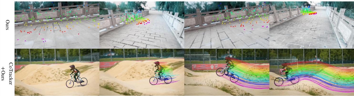
Figure 5. Visualization of Rigid and Dynamic Point Tracking. Top: VGGT’s tracking module $\tau$ outputs keypoint tracks for an unordered set of input images depicting a static scene. Bottom: We finetune the backbone of VGGT to enhance a dynamic point tracker CoTracker [56], which processes sequential inputs.
图 5: 刚性和动态点跟踪的可视化。顶部:VGGT 的跟踪模块 $\tau$ 为描述静态场景的无序输入图像集输出关键点轨迹。底部:我们对 VGGT 的主干网络进行微调,以增强动态点跟踪器 CoTracker [56],该跟踪器处理顺序输入。
Net use ground truth cameras to construct cost volumes.
Net 使用真实相机来构建成本体积。
Our method substantially outperforms DUSt3R, reducing the Overall score from 1.741 to 0.382. More impor- tantly, it achieves results comparable to methods that know ground-truth cameras at test time. The significant performance gains can likely be attributed to our model’s multiimage training scheme that teaches it to reason about multiview triangulation natively, instead of relying on ad hoc alignment procedures, such as in DUSt3R, which only averages multiple pairwise camera triangulation s.
我们的方法显著优于 DUSt3R,将总体得分从 1.741 降低到 0.382。更重要的是,它在测试时取得了与已知真实相机的方法相当的结果。显著的性能提升可能归因于我们模型的多图像训练方案,该方案教会它自然地推理多视图三角测量,而不是依赖于临时对齐程序,例如在 DUSt3R 中,它仅对多个成对相机三角测量进行平均。
4.3. Point Map Estimation
4.3. 点地图估计
We also compare the accuracy of our predicted point cloud to DUSt3R and MASt3R on the ETH3D [97] dataset. For each scene, we randomly sample 10 frames. The predicted point cloud is aligned to the ground truth using the Umeyama [117] algorithm. The results are reported after filtering out invalid points using the official masks. We report Accuracy, Completeness, and Overall (Chamfer distance) for point map estimation. As shown in Tab. 3, although DUSt3R and MASt3R conduct expensive optimization (global alignment–—around 10 seconds per scene), our method still outperforms them significantly in a simple feed-forward regime at only 0.2 seconds per reconstruction.
我们还将预测点云的准确性与 DUSt3R 和 MASt3R 在 ETH3D [97] 数据集上进行了比较。对于每个场景,我们随机采样 10 帧。使用 Umeyama [117] 算法将预测的点云与真实值对齐。结果在使用官方掩码过滤掉无效点后报告。我们报告了点图估计的准确性、完整性和总体(Chamfer 距离)。如表 3 所示,尽管 DUSt3R 和 MASt3R 进行了昂贵的优化(全局对齐——每个场景大约 10 秒),但我们的方法在简单的前馈机制中仍然显著优于它们,每次重建仅需 0.2 秒。
Meanwhile, compared to directly using our estimated point maps, we found that the predictions from our depth and camera heads (i.e., un projecting the predicted depth maps to 3D using the predicted camera parameters) yield higher accuracy. We attribute this to the benefits of decomposing a complex task (point map estimation) into simpler sub problems (depth map and camera prediction), even though camera, depth maps, and point maps are jointly supervised during training.
与此同时,与直接使用我们估计的点云图相比,我们发现从深度和相机头部(即使用预测的相机参数将预测的深度图反投影到3D)得到的预测结果具有更高的准确性。我们将此归因于将复杂任务(点云图估计)分解为更简单的子问题(深度图和相机预测)所带来的好处,尽管在训练过程中相机、深度图和点云图是联合监督的。
We present a qualitative comparison with DUSt3R on inthe-wild scenes in Fig. 3 and further examples in Fig. 4. VGGT outputs high-quality predictions and generalizes well, excelling on challenging out-of-domain examples, such as oil paintings, non-overlapping frames, and scenes with repeating or homogeneous textures like deserts.
我们在图 3 中展示了与 DUSt3R 在野外场景中的定性对比,并在图 4 中提供了更多示例。VGGT 输出了高质量的预测结果,并且具有良好的泛化能力,在具有挑战性的域外示例(如油画、非重叠帧以及具有重复或均匀纹理的场景(如沙漠))中表现出色。
Table 5. Ablation Study for Transformer Backbone on ETH3D. We compare our alternating-attention architecture against two variants: one using only global self-attention and another employing cross-attention.
表 5. ETH3D 上 Transformer 主干的消融研究。我们将交替注意力架构与两种变体进行比较:一种仅使用全局自注意力,另一种采用交叉注意力。
| ETH3D 数据集 | Acc.√ | Comp.√ | Overall√ |
|---|---|---|---|
| 交叉注意力 | 1.287 | 0.835 | 1.061 |
| 仅全局自注意力 | 1.032 | 0.621 | 0.827 |
| 交替注意力 | 0.901 | 0.518 | 0.709 |
4.4. Image Matching
4.4. 图像匹配
Two-view image matching is a widely-explored topic [68, 93, 105] in computer vision. It represents a specific case of rigid point tracking, which is restricted to only two views, and hence a suitable evaluation benchmark to measure our tracking accuracy, even though our model is not specialized for this task. We follow the standard protocol [33, 93] on the ScanNet dataset [18] and report the results in Tab. 4. For each image pair, we extract the matches and use them to estimate an essential matrix, which is then decomposed to a relative camera pose. The final metric is the relative pose accuracy, measured by AUC. For evaluation, we use ALIKED [158] to detect keypoints, treating them as query points ${\bf y}_{q}$ . These are then passed to our tracking branch $\tau$ to find correspondences in the second frame. We adopt the evaluation hyper parameters (e.g., the number of matches, RANSAC thresholds) from Roma [33]. Despite not being explicitly trained for two-view matching, Tab. 4 shows that VGGT achieves the highest accuracy among all baselines.
双视图图像匹配是计算机视觉中一个广泛研究的课题 [68, 93, 105]。它代表了刚性点跟踪的一个特例,仅限于两个视图,因此是一个适合评估我们跟踪精度的基准,尽管我们的模型并非专门为此任务设计。我们遵循 ScanNet 数据集 [18] 上的标准协议 [33, 93],并在表 4 中报告结果。对于每对图像,我们提取匹配点并使用它们来估计一个本质矩阵,然后将其分解为相对相机姿态。最终指标是通过 AUC 测量的相对姿态精度。为了评估,我们使用 ALIKED [158] 检测关键点,并将它们视为查询点 ${\bf y}_{q}$。然后将这些点传递到我们的跟踪分支 $\tau$,以在第二帧中找到对应点。我们采用了 Roma [33] 的评估超参数(例如,匹配数量、RANSAC 阈值)。尽管没有专门针对双视图匹配进行训练,表 4 显示 VGGT 在所有基线中达到了最高的精度。
4.5. Ablation Studies
4.5. 消融研究
Feature Backbone. We first validate the effectiveness of our proposed Alternating-Attention design by comparing it against two alternative attention architectures: (a) global self-attention only, and (b) cross-attention. To ensure a fair comparison, all model variants maintain an identical number of parameters, using a total of $2L$ attention layers. For the cross-attention variant, each frame independently attends to tokens from all other frames, maximizing cross-frame information fusion although significantly increasing the runtime, particularly as the number of input frames grows. The hyper parameters such as the hidden dimension and the number of heads are kept the same. Point map estimation accuracy is chosen as the evaluation metric for our ablation study, as it reflects the model’s joint understanding of scene geometry and camera parameters. Results in Tab. 5 demonstrate that our Alternating-Attention architecture outperforms both baseline variants by a clear margin. Additionally, our other preliminary exploratory experiments consistently showed that architectures using crossattention generally under perform compared to those exclusively employing self-attention.
特征骨干网络。我们首先通过将我们提出的交替注意力设计与两种替代的注意力架构进行比较来验证其有效性:(a) 仅使用全局自注意力,(b) 交叉注意力。为了确保公平比较,所有模型变体保持相同的参数数量,总共使用 $2L$ 个注意力层。对于交叉注意力变体,每一帧独立地关注来自所有其他帧的Token,尽管显著增加了运行时间(特别是随着输入帧数的增加),但最大化了跨帧信息融合。隐藏维度和头数等超参数保持不变。点云图估计精度被选为我们消融研究的评估指标,因为它反映了模型对场景几何和相机参数的联合理解。表 5 中的结果表明,我们的交替注意力架构明显优于两种基线变体。此外,我们的其他初步探索性实验一致表明,使用交叉注意力的架构通常比仅使用自注意力的架构表现较差。
Table 6. Ablation Study for Multi-task Learning, which shows that simultaneous training with camera, depth and track estimation yields the highest accuracy in point map estimation on ETH3D.
表 6. 多任务学习的消融研究,展示了在 ETH3D 上同时进行相机、深度和轨迹估计训练时,点云图估计的准确率最高。
| w. Lcamera | W. Ldepth | w.Ctrack | Acc.↓ | Comp.√ | Overall↓ |
|---|---|---|---|---|---|
| √ | 1.042 | 0.627 | 0.834 | ||
| × | 0.920 | 0.534 | 0.727 | ||
| x | 0.976 | 0.603 | 0.790 | ||
| 0.901 | 0.518 | 0.709 |
Multi-task Learning. We also verify the benefit of training a single network to simultaneously learn multiple 3D quantities, even though these outputs may potentially overlap (e.g., depth maps and camera parameters together can produce point maps). As shown in Tab. 6, there is a noticeable decrease in the accuracy of point map estimation when training without camera, depth, or track estimation. Notably, incorporating camera parameter estimation clearly enhances point map accuracy, whereas depth estimation contributes only marginal improvements.
多任务学习。我们还验证了训练单个网络同时学习多个3D量的好处,尽管这些输出可能存在重叠(例如,深度图和相机参数一起可以生成点图)。如表6所示,在没有相机、深度或轨迹估计的情况下训练时,点图估计的准确性显著下降。值得注意的是,结合相机参数估计明显提高了点图的准确性,而深度估计仅带来边际改进。
4.6. Finetuning for Downstream Tasks
4.6. 下游任务的微调
We now show that the VGGT pre-trained feature extractor can be reused in downstream tasks. We show this for feedforward novel view synthesis and dynamic point tracking.
我们现在展示 VGGT 预训练的特征提取器可以在下游任务中重复使用。我们在前馈新视角合成和动态点跟踪任务中展示了这一点。
Feed-forward Novel View Synthesis is progressing rapidly [8, 43, 49, 53, 108, 126, 140, 155]. Most existing methods take images with known camera parameters as input and predict the target image corresponding to a new camera viewpoint. Instead of relying on an explicit 3D represent ation, we follow LVSM [53] and modify VGGT to directly output the target image. However, we do not assume known camera parameters for the input frames.
前馈式新视角合成 (Feed-forward Novel View Synthesis) 正在快速发展 [8, 43, 49, 53, 108, 126, 140, 155]。大多数现有方法以已知相机参数的图像作为输入,并预测与新相机视角对应的目标图像。我们不依赖于显式的 3D 表示,而是遵循 LVSM [53] 并修改 VGGT 以直接输出目标图像。然而,我们并不假设输入帧的相机参数已知。
We follow the training and evaluation protocol of LVSM closely, e.g., using 4 input views and adopting Plicker rays to represent target viewpoints. We make a simple modification to VGGT. As before, the input images are converted into tokens by DINO. Then, for the target views, we use a convolutional layer to encode their Pluicker ray images into tokens. These tokens, representing both the input images and the target views, are concatenated and processed by the AA transformer. Subsequently, a DPT head is used to regress the RGB colors for the target views. It is important to note that we do not input the Pluicker rays for the source images. Hence, the model is not given the camera parameters for these input frames.
我们紧密遵循 LVSM 的训练和评估协议,例如使用 4 个输入视图并采用 Plicker 光线来表示目标视点。我们对 VGGT 进行了简单的修改。与之前一样,输入图像通过 DINO 转换为 token。然后,对于目标视图,我们使用卷积层将其 Pluicker 光线图像编码为 token。这些表示输入图像和目标视图的 token 被连接起来,并由 AA Transformer 进行处理。随后,使用 DPT 头来回归目标视图的 RGB 颜色。需要注意的是,我们没有为源图像输入 Pluicker 光线。因此,模型没有获得这些输入帧的相机参数。

Figure 6. Qualitative Examples of Novel View Synthesis. The top row shows the input images, the middle row displays the ground truth images from target viewpoints, and the bottom row presents our synthesized images.
图 6: 新视角合成的定性示例。顶部行显示输入图像,中间行显示目标视角的真实图像,底部行展示我们合成的图像。
Table 7. Quantitative comparisons for view synthesis on GSO [28] dataset. Finetuning VGGT for feed-forward novel view synthesis, it demonstrates competitive performance even without knowing camera extrinsic and intrinsic parameters for the input images. Note that ∗ indicates using a small training set (only $20%$ ).
表 7. GSO [28] 数据集上视图合成的定量比较。微调 VGGT 用于前馈新视图合成,即使不知道输入图像的相机外参和内参,也展示了具有竞争力的性能。注意,∗ 表示使用小型训练集(仅 $20%$)。
| 方法 | 已知输入相机 | 尺寸 | PSNR↑ | SSIM↑ | LPIPS↓ |
|---|---|---|---|---|---|
| LGM[110] | √ | 256 | 21.44 | 0.832 | 0.122 |
| GS-LRM[154] | √ | 256 | 29.59 | 0.944 | 0.051 |
| LVSM [53] | 256 | 31.71 | 0.957 | 0.027 | |
| Ours-NVS* | X | 224 | 30.41 | 0.949 | 0.033 |
LVSM was trained on the Objaverse dataset [20]. We use a similar internal dataset of approximately $20%$ the size of Objaverse. Further details on training and evaluation can be found in [53]. As shown in Tab. 7, despite not requiring the input camera parameters and using less training data than LVSM, our model achieves competitive results on the GSO dataset [28]. We expect that better results would be obtained using a larger training dataset. Qualitative examples are shown in Fig. 6.
LVSM 是在 Objaverse 数据集 [20] 上训练的。我们使用了一个类似的内部数据集,其大小约为 Objaverse 的 $20%$。关于训练和评估的更多细节可以在 [53] 中找到。如表 7 所示,尽管不需要输入相机参数且使用的训练数据比 LVSM 少,我们的模型在 GSO 数据集 [28] 上取得了有竞争力的结果。我们预计使用更大的训练数据集会获得更好的结果。定性示例如图 6 所示。
Dynamic Point Tracking has emerged as a highly competitive task in recent years [25, 44, 57, 136], and it serves as another downstream application for our learned features. Following standard practices, we report these point-tracking metrics: Occlusion Accuracy (OA), which comprises the binary accuracy of occlusion predictions; δavvisg, comprising the mean proportion of visible points accurately tracked within a certain pixel threshold; and Average Jaccard (AJ), measuring tracking and occlusion prediction accuracy together.
动态点追踪 (Dynamic Point Tracking) 近年来已成为一项极具竞争力的任务 [25, 44, 57, 136],并且是我们学习到的特征的另一个下游应用。按照标准实践,我们报告了以下点追踪指标:遮挡准确率 (Occlusion Accuracy, OA),包括遮挡预测的二元准确率;δavvisg,包括在一定像素阈值内准确追踪到的可见点的平均比例;以及平均杰卡德系数 (Average Jaccard, AJ),用于同时衡量追踪和遮挡预测的准确性。
Table 8. Dynamic Point Tracking Results on the TAP-Vid benchmarks. Although our model was not designed for dynamic scenes, simply fine-tuning CoTracker with our pretrained weights significantly enhances performance, demonstrating the robustness and effectiveness of our learned features.
表 8: TAP-Vid 基准上的动态点跟踪结果。尽管我们的模型并非为动态场景设计,但仅通过使用我们的预训练权重对 CoTracker 进行微调,性能就显著提升,展示了我们学习到的特征的鲁棒性和有效性。
| 方法 | Kinetics | RGB-S | DAVIS |
|---|---|---|---|
| AJ Svis avg | OA | AJ | |
| TAPTR[63] | 49.0 64.4 85.2 | 60.8 | |
| LocoTrack[13] | 52.9 66.8 85.3 | 69.7 | |
| BootsTAPIR[26] | 54.6 | 68.4 86.5 | 70.8 |
| CoTracker[56] CoTracker+Ours | 57.2 69.0 88.9 | 72.1 84.0 91.6 | 64.7 |
We adapt the state-of-the-art CoTracker2 model [57] by substituting its backbone with our pretrained feature backbone. This is necessary because VGGT is trained on unordered image collections instead of sequential videos. Our backbone predicts the tracking features $T_{i}$ , which replace the outputs of the feature extractor and later enter the rest of the CoTracker2 architecture, that finally predicts the tracks. We finetune the entire modified tracker on Kubric [41]. As illustrated in Tab. 8, the integration of pretrained VGGT significantly enhances CoTracker’s performance on the TAPVid benchmark [23]. For instance, VGGT’s tracking features improve the $\delta_{\mathrm{avg}}^{\mathrm{vis}}$ metric from 78.9 to 84.0 on the TAPVid RGB-S dataset. Despite the TAP-Vid benchmark’s inclusion of videos featuring rapid dynamic motions from various data sources, our model’s strong performance demonstrates the generalization capability of its features, even in scenarios for which it was not explicitly designed.
我们通过将最先进的 CoTracker2 模型 [57] 的骨干网络替换为我们预训练的特征骨干网络来进行适配。这是必要的,因为 VGGT 是在无序图像集合而非序列视频上训练的。我们的骨干网络预测跟踪特征 $T_{i}$,这些特征替代了特征提取器的输出,并随后进入 CoTracker2 架构的其余部分,最终预测轨迹。我们在 Kubric [41] 上对整个修改后的跟踪器进行了微调。如表 8 所示,预训练的 VGGT 的集成显著提升了 CoTracker 在 TAPVid 基准测试 [23] 上的性能。例如,在 TAPVid RGB-S 数据集上,VGGT 的跟踪特征将 $\delta_{\mathrm{avg}}^{\mathrm{vis}}$ 指标从 78.9 提升到 84.0。尽管 TAP-Vid 基准测试包含了来自各种数据源的快速动态运动视频,我们模型的强大性能展示了其特征的泛化能力,即使是在未明确设计的场景中也是如此。
5. Discussions
5. 讨论
Limitations. While our method exhibits strong generalization to diverse in-the-wild scenes, several limitations remain. First, the current model does not support fisheye or panoramic images. Additionally, reconstruction performance drops under conditions involving extreme input rotations. Moreover, although our model handles scenes with minor non-rigid motions, it fails in scenarios involving substantial non-rigid deformation.
局限性。虽然我们的方法在多样化的野外场景中表现出强大的泛化能力,但仍存在一些局限性。首先,当前模型不支持鱼眼或全景图像。此外,在输入旋转极端的情况下,重建性能会下降。此外,尽管我们的模型能够处理具有轻微非刚性运动的场景,但在涉及大量非刚性变形的情况下会失效。
However, an important advantage of our approach is its flexibility and ease of adaptation. Addressing these limitations can be straightforwardly achieved by fine-tuning the model on targeted datasets with minimal architectural modifications. This adaptability clearly distinguishes our method from existing approaches, which typically require extensive re-engineering during test-time optimization to accommodate such specialized scenarios.
然而,我们方法的一个重要优势在于其灵活性和易于适应性。通过在有针对性数据集上进行微调,只需最少的架构修改即可直接解决这些限制。这种适应性明显将我们的方法与现有方法区分开来,后者通常需要在测试时优化期间进行大量重新设计以适应此类专门场景。
Table 9. Runtime and peak GPU memory usage across different numbers of input frames. Runtime is measured in seconds, and GPU memory usage is reported in gigabytes.
表 9. 不同输入帧数下的运行时间和峰值 GPU 内存使用情况。运行时间以秒为单位,GPU 内存使用情况以千兆字节为单位报告。
| 输入帧数 | 2 | 4 | 8 | 10 | 20 | 50 | 100 | 200 |
|---|---|---|---|---|---|---|---|---|
| 时间 (秒) | 0.04 | 0.05 | 0.07 | 0.11 | 0.14 | 0.31 | 1.04 | 3.12 |
| 内存 (GB) | 1.88 | 2.07 | 2.45 | 3.23 | 3.63 | 5.58 | 11.41 | 21.15 |
Runtime and Memory. As shown in Tab. 9, we evaluate inference runtime and peak GPU memory usage of the feature backbone when processing varying numbers of input frames. Measurements are conducted using a single NVIDIA H100 GPU with flash attention v3 [98]. Images have a resolution of $336\times518$ .
运行时和内存。如表 9 所示,我们评估了在处理不同数量的输入帧时特征骨干网络的推理运行时间和峰值 GPU 内存使用情况。测量使用单个 NVIDIA H100 GPU 和 flash attention v3 [98] 进行。图像分辨率为 $336\times518$。
We focus on the cost associated with the feature backbone since users may select different branch combinations depending on their specific requirements and available resources. The camera head is lightweight, typically accounting for approximately $5%$ of the runtime and about $2%$ of the GPU memory used by the feature backbone. A DPT head uses an average of 0.03 seconds and 0.2 GB GPU memory per frame.
我们关注与特征主干相关的成本,因为用户可能会根据其特定需求和可用资源选择不同的分支组合。相机头部分较为轻量,通常占特征主干运行时间的约 $5%$,以及占用的 GPU 内存的约 $2%$。一个 DPT 头每帧平均使用 0.03 秒和 0.2 GB 的 GPU 内存。
When GPU memory is sufficient, multiple frames can be processed efficiently in a single forward pass. At the same time, in our model, inter-frame relationships are handled only within the feature backbone, and the DPT heads make independent predictions per frame. Therefore, users constrained by GPU resources may perform predictions frame by frame. We leave this trade-off to the user’s discretion.
当 GPU 内存充足时,可以在一次前向传递中高效处理多个帧。同时,在我们的模型中,帧间关系仅在特征骨干网络内处理,DPT 头对每一帧进行独立预测。因此,受 GPU 资源限制的用户可以逐帧进行预测。我们将这种权衡留给用户自行决定。
We recognize that a naive implementation of global selfattention can be highly memory-intensive with a large number of tokens. Savings or accelerations can be achieved by employing techniques used in large language model (LLM) deployments. For instance, Fast3R [141] employs Tensor Parallelism to accelerate inference with multiple GPUs, which can be directly applied to our model.
我们认识到,全局自注意力(global self-attention)的简单实现在处理大量 Token 时可能会非常消耗内存。通过采用大语言模型(LLM)部署中的技术,可以实现内存节省或加速。例如,Fast3R [141] 使用 Tensor Parallelism 来加速多 GPU 推理,这可以直接应用于我们的模型。
Patch if ying. As discussed in Sec. 3.2, we have explored the method of patch if ying images into tokens by utilizing either a $14\times14$ convolutional layer or a pretrained DINOv2 model. Empirical results indicate that the DINOv2 model provides better performance; moreover, it ensures much more stable training, particularly in the initial stages. The DINOv2 model is also less sensitive to variations in hyper parameters such as learning rate or momentum. Consequently, we have chosen DINOv2 as the default method for patch if ying in our model.
Patch if ying。正如第 3.2 节所讨论的,我们探索了通过使用 $14\times14$ 卷积层或预训练的 DINOv2 模型将图像 patch if ying 为 token 的方法。实验结果表明,DINOv2 模型提供了更好的性能;此外,它确保了更稳定的训练,特别是在初始阶段。DINOv2 模型对超参数(如学习率或动量)的变化也不太敏感。因此,我们选择 DINOv2 作为我们模型中 patch if ying 的默认方法。
Differentiable BA. We also explored the idea of using differentiable bundle adjustment as in VGGSfM [125]. In small-scale preliminary experiments, differentiable BA demonstrated promising performance. However, a bottleneck is its computational cost during training. Enabling differentiable BA in PyTorch using Theseus [85] typically makes each training step roughly 4 times slower, which is expensive for large-scale training. While customizing a framework to expedite training could be a potential solution, it falls outside the scope of this work. Thus, we opted not to include differentiable BA in this work, but we recognize it as a promising direction for large-scale unsupervised training, as it can serve as an effective supervision signal in scenarios lacking explicit 3D annotations.
可微BA。我们还探索了像VGGSfM [125]那样使用可微束调整的想法。在小规模的初步实验中,可微BA展示了良好的性能。然而,其瓶颈在于训练期间的计算成本。使用Theseus [85]在PyTorch中启用可微BA通常会使每个训练步骤大约慢4倍,这对于大规模训练来说是昂贵的。虽然定制框架以加速训练可能是一个潜在的解决方案,但这超出了本工作的范围。因此,我们选择不在本工作中包含可微BA,但我们认为它是大规模无监督训练的一个有前景的方向,因为它可以在缺乏显式3D注释的场景中作为有效的监督信号。
Single-view Reconstruction. Unlike systems like DUSt3R and MASt3R that have to duplicate an image to create a pair, our model architecture inherently supports the input of a single image. In this case, global attention simply transitions to frame-wise attention. Although our model was not explicitly trained for single-view reconstruction, it demonstrates surprisingly good results. Some examples can be found in Fig. 3 and Fig. 7. We strongly encourage trying our demo for better visualization.
单视图重建。与DUSt3R和MASt3R等系统需要复制图像以创建图像对不同,我们的模型架构天然支持单张图像的输入。在这种情况下,全局注意力机制会简单地转变为帧级注意力。尽管我们的模型并未专门针对单视图重建进行训练,但它展示了出人意料的好效果。一些示例可以在图3和图7中找到。我们强烈建议尝试我们的演示以获得更好的可视化效果。
Normalizing Prediction. As discussed in Sec. 3.4, our approach normalizes the ground truth using the average Euclidean distance of the 3D points. While some methods, such as DUSt3R, also apply such normalization to network predictions, our findings suggest that it is neither necessary for convergence nor advantageous for final model performance. Furthermore, it tends to introduce additional instability during the training phase.
归一化预测。如第3.4节所述,我们的方法使用3D点的平均欧几里得距离对真实值进行归一化。虽然一些方法(如DUSt3R)也对网络预测应用了这种归一化,但我们的研究结果表明,这种归一化既不是收敛的必要条件,也不会提高最终模型的性能。此外,它往往会在训练阶段引入额外的不稳定性。
6. Conclusions
6. 结论
We present Visual Geometry Grounded Transformer (VGGT), a feed-forward neural network that can directly estimate all key 3D scene properties for hundreds of input views. It achieves state-of-the-art results in multiple 3D tasks, including camera parameter estimation, multiview depth estimation, dense point cloud reconstruction, and 3D point tracking. Our simple, neural-first approach departs from traditional visual geometry-based methods, which rely on optimization and post-processing to obtain accurate and task-specific results. The simplicity and efficiency of our approach make it well-suited for real-time applications, which is another benefit over optimization-based approaches.
我们提出了视觉几何基础Transformer (VGGT),这是一种前馈神经网络,能够直接估计数百个输入视图的所有关键3D场景属性。它在多个3D任务中取得了最先进的结果,包括相机参数估计、多视图深度估计、密集点云重建和3D点跟踪。我们这种简单的、以神经网络为先的方法与传统基于视觉几何的方法不同,后者依赖于优化和后处理来获得准确且特定于任务的结果。我们方法的简单性和效率使其非常适合实时应用,这是相对于基于优化的方法的另一个优势。
Appendix
附录
In the Appendix, we provide the following:
在附录中,我们提供了以下内容:
• formal definitions of key terms in Appendix A. • comprehensive implementation details, including architecture and training hyper parameters in Appendix B. • additional experiments and discussions in Appendix C. • qualitative examples of single-view reconstruction in Appendix D. • an expanded review of related works in Appendix E.
• 关键术语的正式定义见附录 A。
• 全面的实现细节,包括架构和训练超参数见附录 B。
• 额外的实验和讨论见附录 C。
• 单视图重建的定性示例见附录 D。
• 相关工作的扩展综述见附录 E。
A. Formal Definitions
A. 正式定义
In this section, we provide additional formal definitions that further ground the method section.
在本节中,我们提供了额外的正式定义,以进一步夯实方法部分的基础。
The camera extrinsics are defined in relation to the world reference frame, which we take to be the coordinate system of the first camera. We thus introduce two functions. The first function $\gamma(\mathbf{g},\mathbf{p})=\mathbf{p}^{\prime}$ applies the rigid transformation encoded by $\mathbf{g}$ to a point $\mathbf{p}$ in the world reference frame to obtain the corresponding point $\mathbf{p^{\prime}}$ in the camera reference frame. The second function $\pi(\mathbf{g},\mathbf{p})=\mathbf{y}$ further applies perspective projection, mapping the 3D point $\mathbf{p}$ to a 2D image point y. We also denote the depth of the point as observed from the camera $\mathbf{g}$ by $\pi^{\mathrm{D}}(\mathbf{g},\mathbf{p})=d\in\mathbb{R}^{+}$ .
相机的外参是相对于世界参考系定义的,我们将其视为第一个相机的坐标系。因此,我们引入了两个函数。第一个函数 $\gamma(\mathbf{g},\mathbf{p})=\mathbf{p}^{\prime}$ 将 $\mathbf{g}$ 编码的刚体变换应用于世界参考系中的点 $\mathbf{p}$,以获得相机参考系中的对应点 $\mathbf{p^{\prime}}$。第二个函数 $\pi(\mathbf{g},\mathbf{p})=\mathbf{y}$ 进一步应用透视投影,将 3D 点 $\mathbf{p}$ 映射到 2D 图像点 y。我们还表示从相机 $\mathbf{g}$ 观察到的点的深度为 $\pi^{\mathrm{D}}(\mathbf{g},\mathbf{p})=d\in\mathbb{R}^{+}$。
We model the scene as a collection of regular surfaces $S_{i}\subset\mathbb{R}^{3}$ . We make this a function of the $i$ -th input image as the scene can change over time [151]. The depth at pixel location $\mathbf{y}\in\mathcal{I}(I_{i})$ is defined as the minimum depth of any 3D point $\mathbf{p}$ in the scene that projects to y, i.e., $D_{i}(\mathbf{y})=$ $\operatorname*{min}{\pi^{D}(\mathbf{g}{i},\mathbf{p}):\mathbf{p}\in S{i}\wedge\pi(\mathbf{g}_{i},\mathbf{p})=\mathbf{y}}$ . The point at pixel location $\mathbf{y}$ is then given by $P_{i}(\mathbf{y})=\gamma(\mathbf{g},\mathbf{p})$ , where $\mathbf{p}\in S_{i}$ is the 3D point that minimizes the expression above, i.e. $\mathbf{p}\in S_{i}\wedge\pi(\mathbf{g}_{i},\mathbf{p})=\mathbf{y}\wedge\pi^{D}(\mathbf{g}_{i},\mathbf{p})=D_{i}(\mathbf{y}).$
我们将场景建模为一组规则曲面 $S_{i}\subset\mathbb{R}^{3}$ 的集合。由于场景可能随时间变化 [151],我们将其作为第 $i$ 个输入图像的函数。像素位置 $\mathbf{y}\in\mathcal{I}(I_{i})$ 处的深度定义为投影到 y 的任何 3D 点 $\mathbf{p}$ 的最小深度,即 $D_{i}(\mathbf{y})=$ $\operatorname*{min}{\pi^{D}(\mathbf{g}{i},\mathbf{p}):\mathbf{p}\in S{i}\wedge\pi(\mathbf{g}_{i},\mathbf{p})=\mathbf{y}}$ 。像素位置 $\mathbf{y}$ 处的点由 $P_{i}(\mathbf{y})=\gamma(\mathbf{g},\mathbf{p})$ 给出,其中 $\mathbf{p}\in S_{i}$ 是使上述表达式最小化的 3D 点,即 $\mathbf{p}\in S_{i}\wedge\pi(\mathbf{g}_{i},\mathbf{p})=\mathbf{y}\wedge\pi^{D}(\mathbf{g}_{i},\mathbf{p})=D_{i}(\mathbf{y}).$
B. Implementation Details
B. 实现细节
Architecture. As mentioned in the main paper, VGGT consists of 24 attention blocks, each block equipped with one frame-wise self-attention layer and one global selfattention layer. Following the ViT-L model used in DINOv2 [78], each attention layer is configured with a feature dimension of 1024 and employs 16 heads. We use the official implementation of the attention layer from PyTorch, i.e., torch.nn.Multi head Attention, with flash attention enabled. To stabilize training, we also use QKNorm [48] and LayerScale [115] for each attention layer. The value of LayerScale is initialized with 0.01. For image token iz ation, we use DINOv2 [78] and add positional embedding. As in [143], we feed the tokens from the 4-th, 11-th, 17-th, and 23-rd block into DPT [87] for upsampling.
架构。如主论文所述,VGGT 由 24 个注意力块组成,每个块配备一个帧级自注意力层和一个全局自注意力层。根据 DINOv2 [78] 中使用的 ViT-L 模型,每个注意力层的特征维度配置为 1024,并使用 16 个头。我们使用 PyTorch 官方实现的注意力层,即 torch.nn.MultiheadAttention,并启用了 flash attention。为了稳定训练,我们还为每个注意力层使用了 QKNorm [48] 和 LayerScale [115]。LayerScale 的值初始化为 0.01。对于图像 Token 化,我们使用 DINOv2 [78] 并添加位置嵌入。如 [143] 所述,我们将第 4、11、17 和 23 块的 Token 输入到 DPT [87] 中进行上采样。
Training. To form a training batch, we first choose a random training dataset (each dataset has a different yet approximate ly similar weight, as in [129]), and from the dataset, we then sample a random scene (uniformly). During the training phase, we select between 2 and 24 frames per scene while maintaining the constant total of 48 frames within each batch. For training, we use the respective training sets of each dataset. We exclude training sequences containing fewer than 24 frames. RGB frames, depth maps, and point maps are first isotropic ally resized, so the longer size has 518 pixels. Then, we crop the shorter dimension (around the principal point) to a size between 168 and 518 pixels while remaining a multiple of the 14-pixel patch size. It is worth mentioning that we apply aggressive color augmentation independently across each frame within the same scene, enhancing the model’s robustness to varying lighting conditions. We build ground truth tracks following [33, 105, 125], which unprojects depth maps to 3D, reprojects points to target frames, and retains correspondences where re projected depths match target depth maps. Frames with low similarity to the query frame are excluded during batch sampling. In rare cases with no valid correspondences, the tracking loss is omitted.
训练。为了形成一个训练批次,我们首先随机选择一个训练数据集(每个数据集有不同的但大致相似的权重,如 [129] 所述),然后从数据集中均匀地随机采样一个场景。在训练阶段,我们为每个场景选择 2 到 24 帧,同时保持每个批次中总帧数为 48 帧。对于训练,我们使用每个数据集的相应训练集。我们排除包含少于 24 帧的训练序列。RGB 帧、深度图和点图首先进行各向同性调整大小,使较长边的尺寸为 518 像素。然后,我们裁剪较短边(围绕主点)至 168 到 518 像素之间的尺寸,同时保持为 14 像素块大小的倍数。值得一提的是,我们在同一场景内的每一帧上独立应用了强烈的颜色增强,以增强模型在不同光照条件下的鲁棒性。我们按照 [33, 105, 125] 的方法构建地面实况轨迹,将深度图反投影到 3D 空间,将点重新投影到目标帧,并保留重新投影的深度与目标深度图匹配的对应关系。在批次采样过程中,排除与查询帧相似度较低的帧。在极少数没有有效对应关系的情况下,跟踪损失会被省略。
C. Additional Experiments
C. 额外实验
Camera Pose Estimation on IMC We also evaluate using the Image Matching Challenge (IMC) [54], a camera pose estimation benchmark focusing on photo tourism data. Until recently, the benchmark was dominated by classical incremental SfM methods [94].
在IMC上进行相机姿态估计
我们还使用图像匹配挑战赛 (Image Matching Challenge, IMC) [54] 进行评估,这是一个专注于照片旅游数据的相机姿态估计基准。直到最近,该基准一直由经典的增量式SfM方法 [94] 主导。
Baselines. We evaluate two flavors of our model: VGGT and $\mathrm{VGGT}+\mathrm{BA}$ . VGGT directly outputs camera pose estimates, while $\mathrm{VGGT}+\mathrm{BA}$ refines the estimates using an additional Bundle Adjustment stage. We compare to the classical incremental SfM methods such as [66, 94] and to recently-proposed deep methods. Specifically, recently VGGSfM [125] provided the first end-to-end trained deep method that outperformed incremental SfM on the challenging photo tourism datasets.
基线。我们评估了两种模型变体:VGGT 和 $\mathrm{VGGT}+\mathrm{BA}$。VGGT 直接输出相机姿态估计,而 $\mathrm{VGGT}+\mathrm{BA}$ 则通过额外的 Bundle Adjustment 阶段来优化估计结果。我们与经典的增量式 SfM 方法(如 [66, 94])以及最近提出的深度学习方法进行了比较。具体来说,VGGSfM [125] 最近提出了第一个端到端训练的深度方法,在具有挑战性的照片旅游数据集上超越了增量式 SfM。
Besides VGGSfM, we additionally compare to recently popularized DUSt3R [129] and MASt3R [62]. It is important to note that DUSt3R and MASt3R utilized a substantial portion of the MegaDepth dataset for training, only excluding scenes 0015 and 0022. The MegaDepth scenes employed in their training have some overlap with the IMC benchmark, although the images are not identical; the same scenes are present in both datasets. For instance, the MegaDepth scene 0024 corresponds to the British Museum, while the British Museum is also a scene in the IMC benchmark. For an apples-to-apples comparison, we adopt the same training split as DUSt3R and MASt3R. In the main paper, to ensure a fair comparison on ScanNet-1500, we exclude the corresponding ScanNet scenes from our training.
除了 VGGSfM,我们还与最近流行的 DUSt3R [129] 和 MASt3R [62] 进行了比较。需要注意的是,DUSt3R 和 MASt3R 使用了 MegaDepth 数据集的大部分进行训练,仅排除了场景 0015 和 0022。他们训练中使用的 MegaDepth 场景与 IMC 基准测试有一些重叠,尽管图像并不完全相同;两个数据集中都存在相同的场景。例如,MegaDepth 场景 0024 对应的是大英博物馆,而大英博物馆也是 IMC 基准测试中的一个场景。为了进行公平的比较,我们采用了与 DUSt3R 和 MASt3R 相同的训练划分。在主论文中,为了确保在 ScanNet-1500 上进行公平比较,我们从训练中排除了相应的 ScanNet 场景。
Results. Table 10 contains the results of our evaluation. Although photo tourism data is the traditional focus of SfM methods, our VGGT’s feed-forward performance is on par with the state-of-the-art VGGSfMv2 with $\operatorname{AUC@10}$ of 71.26 versus 76.82, while being significantly faster (0.2 vs. 10 seconds per scene). Remarkably, VGGT outperforms both MASt3R [62] and DUSt3R [129] significantly across all accuracy thresholds while being much faster. This is because MASt3R’s and DUSt3R’s feed-forward predictions can only process pairs of frames and, hence, require a costly global alignment step. Additionally, with bundle adjustment, $\mathrm{VGGT}+\mathrm{BA}$ further improves drastically, achieving state-of-the-art performance on IMC, raising AUC $@10$ from 71.26 to 84.91, and raising $\mathrm{AUC@3}$ from 39.23 to 66.37. Note that our model directly predicts 3D points, which can serve as the initialization for BA. This eliminates the need for triangulation and iterative refinement of BA as in [125]. As a result, $\mathrm{VGGT}+\mathrm{BA}$ is much faster than [125].
结果。表 10 包含了我们的评估结果。尽管照片旅游数据是 SfM 方法的传统关注点,但我们的 VGGT 的前馈性能与最先进的 VGGSfMv2 相当,$\operatorname{AUC@10}$ 为 71.26 对 76.82,同时速度显著更快(每场景 0.2 秒对 10 秒)。值得注意的是,VGGT 在所有精度阈值上均显著优于 MASt3R [62] 和 DUSt3R [129],同时速度更快。这是因为 MASt3R 和 DUSt3R 的前馈预测只能处理成对的帧,因此需要昂贵的全局对齐步骤。此外,通过捆绑调整,$\mathrm{VGGT}+\mathrm{BA}$ 进一步大幅提升,在 IMC 上实现了最先进的性能,将 AUC $@10$ 从 71.26 提高到 84.91,并将 $\mathrm{AUC@3}$ 从 39.23 提高到 66.37。请注意,我们的模型直接预测 3D 点,这些点可以作为 BA 的初始化。这消除了如 [125] 中所需的三角测量和 BA 的迭代优化。因此,$\mathrm{VGGT}+\mathrm{BA}$ 比 [125] 快得多。
Table 10. Camera Pose Estimation on IMC [54]. Our method achieves state-of-the-art performance on the challenging phototropism data, outperforming VGGSfMv2 [125] which ranked first on the latest CVPR’24 IMC Challenge in camera pose (rotation and translation) estimation.
表 10. IMC [54] 上的相机姿态估计。我们的方法在具有挑战性的向光性数据上实现了最先进的性能,超越了在最新的 CVPR’24 IMC 挑战赛中相机姿态(旋转和平移)估计排名第一的 VGGSfMv2 [125]。
| 方法 | 测试时间优化 | AUC@3° | AUC@5° | AUC@10° | 运行时间 |
|---|---|---|---|---|---|
| COLMAP(SIFT+NN)[94] | 23.58 | 32.66 | 44.79 | >10s | |
| PixSfM (SIFT + NN) [66] | 25.54 | 34.80 | 46.73 | >20s | |
| PixSfM (LoFTR) [66] | 44.06 | 56.16 | 69.61 | >20s | |
| PixSfM (SP+ SG) [66] | 45.19 | 57.22 | 70.47 | >20s | |
| DFSfM (LoFTR)[47] | 46.55 | 58.74 | 72.19 | >10s | |
| DUSt3R[129] | 13.46 | 21.24 | 35.62 | ~7s | |
| MASt3R[62] | 30.25 | 46.79 | 57.42 | ~9s | |
| VGGSfM[125] | 45.23 | 58.89 | 73.92 | ~6s | |
| VGGSfMv2[125] | 59.32 | 67.78 | 76.82 | ~10s | |
| VGGT(ours) | 39.23 | 52.74 | 71.26 | 0.2s | |
| VGGT+BA (ours) | 66.37 | 75.16 | 84.91 | 1.8s |
D. Qualitative Examples
D. 定性示例
We further present qualitative examples of single-view reconstruction in Fig. 7.
我们进一步在图 7 中展示了单视图重建的定性示例。
E. Related Work
E. 相关工作
In this section, we discuss additional related works.
在本节中,我们将讨论其他相关研究工作。
Vision Transformers. The Transformer architecture was initially proposed for language processing tasks [6, 22, 120]. It was later introduced to the computer vision community by ViT [27], sparking widespread adoption. Vision Transformers and their variants have since become dominant in the design of architectures for various computer vision tasks [4, 12, 83, 137], thanks to their simplicity, high capacity, flexibility, and ability to capture long-range dependencies.
Vision Transformers。Transformer 架构最初是为语言处理任务提出的 [6, 22, 120]。后来,ViT [27] 将其引入计算机视觉领域,引发了广泛的应用。由于其简单性、高容量、灵活性以及捕捉长距离依赖关系的能力,Vision Transformers 及其变体在各种计算机视觉任务的架构设计中占据了主导地位 [4, 12, 83, 137]。
DeiT [114] demonstrated that Vision Transformers can be effectively trained on datasets like ImageNet using strong data augmentation strategies. DINO [10] revealed intriguing properties of features learned by Vision Transformers in a self-supervised manner. CaiT [115] introduced layer scaling to address the challenges of training deeper Vision Transformers, effectively mitigating gradient-related issues. Further, techniques such as QKNorm [48, 150] have been proposed to stabilize the training process. Additionally, [138] also explores the dynamics between frame-wise and global attention modules in object tracking, though using cross-attention.
DeiT [114] 展示了通过强大的数据增强策略,Vision Transformer 可以在 ImageNet 等数据集上有效训练。DINO [10] 揭示了通过自监督方式学习的 Vision Transformer 特征的有趣特性。CaiT [115] 引入了层缩放技术,以解决训练更深层 Vision Transformer 的挑战,有效缓解了梯度相关问题。此外,QKNorm [48, 150] 等技术被提出以稳定训练过程。另外,[138] 还探索了在目标跟踪中帧级和全局注意力模块之间的动态关系,尽管使用了交叉注意力。

Figure 7. Single-view Reconstruction by Point Map Estimation. Unlike DUSt3R, which requires duplicating an image into a pair, our model can predict the point map from a single input image. It demonstrates strong generalization to unseen real-world images.
图 7: 通过点云图估计的单视图重建。与需要将图像复制成对的 DUSt3R 不同,我们的模型可以从单个输入图像预测点云图。它展示了对未见过的真实世界图像的强大泛化能力。
Camera Pose Estimation. Estimating camera poses from multi-view images is a crucial problem in 3D computer vision. Over the last decades, Structure from Motion (SfM) has emerged as the dominant approach [46], whether incremental [2, 36, 94, 103, 134] or global [3, 14–17, 52, 73, 79, 81, 90, 106]. Recently, a set of methods treat camera pose estimation as a regression problem [65, 100, 109, 112, 113, 118, 122, 123, 131, 152, 153, 160], which show promising results under the sparse-view setting. AceZero [5] further proposes to regress 3D scene coordinates and FlowMap [101] focuses on depth maps, as intermediates for camera prediction. Instead, VGGSfM [125] simplifies the classical SfM pipeline to a differentiable framework, demonstrating exceptional performance, particularly with photo tourism datasets. At the same time, DUSt3R [62, 129] introduces an approach to learn pixel-aligned point map, and hence camera poses can be recovered by simple alignment. This paradigm shift has garnered considerable interest as the point map, an over-parameterized representation, offers seamless integration with various downstream applications, such as 3D Gaussian splatting.
相机姿态估计。从多视角图像中估计相机姿态是3D计算机视觉中的一个关键问题。在过去的几十年里,运动恢复结构 (Structure from Motion, SfM) 已成为主导方法 [46],无论是增量式 [2, 36, 94, 103, 134] 还是全局式 [3, 14–17, 52, 73, 79, 81, 90, 106]。最近,一些方法将相机姿态估计视为回归问题 [65, 100, 109, 112, 113, 118, 122, 123, 131, 152, 153, 160],在稀疏视角设置下表现出色。AceZero [5] 进一步提出回归3D场景坐标,而FlowMap [101] 则专注于深度图,作为相机预测的中间步骤。相反,VGGSfM [125] 将经典的SfM流程简化为一个可微框架,展示了卓越的性能,特别是在照片旅游数据集上。同时,DUSt3R [62, 129] 引入了一种学习像素对齐点图的方法,因此可以通过简单的对齐恢复相机姿态。这种范式转变引起了广泛关注,因为点图作为一种过参数化表示,可以与各种下游应用(如3D高斯泼溅)无缝集成。