MobileNetV2: Inverted Residuals and Linear Bottlenecks
论文中英文对照合集 : https://aiqianji.com/blog/articles
ABSTRACT
In this paper we describe a new mobile architecture, MobileNetV2, that improves the state of the art performance of mobile models on multiple tasks and benchmarks as well as across a spectrum of different model sizes. We also describe efficient ways of applying these mobile models to object detection in a novel framework we call SSDLite. Additionally, we demonstrate how to build mobile semantic segmentation models through a reduced form of DeepLabv3 which we call Mobile DeepLabv3.
The MobileNetV2 architecture is based on an inverted residual structure where the input and output of the residual block are thin bottleneck layers opposite to traditional residual models which use expanded representations in the input and output [1]. MobileNetV2 uses lightweight depthwise convolutions to filter features in the intermediate expansion layer. Additionally, we find that it is important to remove non-linearities in the narrow layers in order to maintain representational power. We demonstrate that this improves performance and provide an intuition that led to this design. Finally, our approach allows decoupling of the input/output domains from the expressiveness of the transformation, which provides a convenient framework for further analysis. We measure our performance on ImageNet [2] classification, COCO object detection [3], VOC image segmentation [4]. We evaluate the trade-offs between accuracy, and number of operations measured by multiply-adds (MAdd), as well as the number of parameters.
摘要
在本文中,我们描述了一种新的移动架构MobileNetV2,该架构提高了移动模型在多个任务和多个基准数据集上以及在不同模型尺寸范围内的最佳性能。我们还描述了在我们称之为SSDLite的新框架中将这些移动模型应用于目标检测的有效方法。此外,我们还演示了如何通过DeepLabv3的简化形式,我们称之为Mobile DeepLabv3来构建移动语义分割模型。
MobileNetV2架构基于倒置的残差结构,其中快捷连接位于窄的瓶颈层之间。中间展开层使用轻量级的深度卷积作为非线性源来过滤特征。此外,我们发现为了保持表示能力,去除窄层中的非线性是非常重要的。我们证实了这可以提高性能并提供了产生此设计的直觉。
最后,我们的方法允许将输入/输出域与变换的表现力解耦,这为进一步分析提供了便利的框架。我们在ImageNet分类,COCO目标检测,VOC图像分割上评估了我们的性能。我们评估了在精度、通过乘加(MAdd)度量的操作次数,以及实际的延迟和参数的数量之间的权衡。
1INTRODUCTION
Neural networks have revolutionized many areas of machine intelligence, enabling superhuman accuracy for challenging image recognition tasks. However, the drive to improve accuracy often comes at a cost: modern state of the art networks require high computational resources beyond the capabilities of many mobile and embedded applications.
This paper introduces a new neural network architecture that is specifically tailored for mobile and resource constrained environments. Our network pushes the state of the art for mobile tailored computer vision models, by significantly decreasing the number of operations and memory needed while retaining the same accuracy.
Our main contribution is a novel layer module: the inverted residual with linear bottleneck. This module takes as an input a low-dimensional compressed representation which is first expanded to high dimension and filtered with a lightweight depthwise convolution. Features are subsequently projected back to a low-dimensional representation with a linear convolution.
This module can be efficiently implemented using standard operations in any modern framework and allows our models to beat state of the art along multiple performance points using standard benchmarks. Furthermore, this convolutional module is particularly suitable for mobile designs, because it allows to significantly reduce the memory footprint needed during inference by never fully materializing large intermediate tensors. This reduces the need for main memory access in many embedded hardware designs, that provide small amounts of very fast software controlled cache memory.
1. 引言
神经网络已经彻底改变了机器智能的许多领域,使具有挑战性的图像识别任务获得了超过常人的准确性。然而,提高准确性的驱动力往往需要付出代价:现代先进网络需要超出许多移动和嵌入式应用能力之外的高计算资源。
本文介绍了一种专为移动和资源受限环境量身定制的新型神经网络架构。我们的网络通过显著减少所需操作和内存的数量,同时保持相同的精度推进了移动定制计算机视觉模型的最新水平。
我们的主要贡献是一个新的层模块:具有线性瓶颈的倒置残差。该模块将输入的低维压缩表示首先扩展到高维并用轻量级深度卷积进行过滤。随后用线性卷积将特征投影回低维表示。官方实现可作为[4]中TensorFlow-Slim模型库的一部分。
这个模块可以使用任何现代框架中的标准操作来高效地实现,并允许我们的模型使用标准基线沿多个性能点击败最先进的技术。此外,这种卷积模块特别适用于移动设计,因为它可以通过从不完全实现大型中间张量来显著减少推断过程中所需的内存占用。这减少了许多嵌入式硬件设计中对主存储器访问的需求,这些设计提供了少量高速软件控制缓存。
2 RELATED WORK
Tuning deep neural architectures to strike an optimal balance between accuracy and performance has been an area of active research for the last several years. Both manual architecture search and improvements in training algorithms, carried out by numerous teams has led to creation of such well-known models as AlexNet [5], VGGNet [6], GoogLeNet [7], and ResNet [1]. Recently there has been lots of progress in algorithmic architecture exploration included hyper-parameter optimization [8, 9, 10] as well as various methods of network pruning [11, 12, 13, 14, 15, 16] and connectivity learning [17, 18]. A substantial amount of work has also been dedicated to changing the connectivity structure of the internal convolutional blocks such as in ShuffleNet [19] or introducing sparsity [20] and others [21].
Recently, [22, 23, 24, 25], opened up a new direction of bringing optimization methods including genetic algorithms and reinforcement learning to architectural search. However one drawback is that the resulting networks end up very complex. In this paper, we pursue the goal of developing better intuition about how neural networks operate and use that to guide the simplest possible network design. Our approach should be seen as complimentary to the one described in [22] and related work. In this vein our approach is similar to those taken by [19, 21] and allows to further improve the performance, while providing a glimpse on its internal operation. Our network design is based on MobileNetV1 [26]. It retains its simplicity and significantly improves its accuracy, achieving state of the art on multiple image classification and detection tasks for mobile applications.
2. 相关工作
调整深层神经架构以在精确性和性能之间达到最佳平衡已成为过去几年研究活跃的一个领域。由许多团队进行的手动架构搜索和训练算法的改进,已经比早期的设计(如AlexNet[5],VGGNet [6],GoogLeNet[7]和ResNet[8])有了显著的改进。最近在算法架构探索方面取得了很多进展,包括超参数优化[9,10,11]、各种网络修剪方法[12,13,14,15,16,17]和连接学习[18,19]。 也有大量的工作致力于改变内部卷积块的连接结构如ShuffleNet[20]或引入稀疏性[21]和其他[22]。
最近,[23,24,25,26]开辟了了一个新的方向,将遗传算法和强化学习等优化方法带入架构搜索。然而,一个缺点是最终所得到的网络非常复杂。在本文中,我们追求的目标是发展了解神经网络如何运行的更好直觉,并使用它来指导最简单可能的网络设计。我们的方法应该被视为[23]中描述的方法和相关工作的补充。在这种情况下,我们的方法与[20,22]所采用的方法类似,并且可以进一步提高性能,同时可以一睹其内部的运行。我们的网络设计基于MobileNetV1[27]。它保留了其简单性,并且不需要任何特殊的运算符,同时显著提高了它的准确性,为移动应用实现了在多种图像分类和检测任务上的最新技术。
3. PRELIMINARIES, DISCUSSION AND INTUITION 准备,讨论和直觉
3.1. DEPTHWISE SEPARABLE CONVOLUTIONS 深度可分卷积
Depthwise Separable Convolutions are a key building block for many efficient neural network architectures [26, 27, 19] and we use them in the present work as well. The basic idea is to replace a full convolutional operator with a factorized version that splits convolution into two separate layers. The first layer is called a depthwise convolution, it performs lightweight filtering by applying a single convolutional filter per input channel. The second layer is a 1×1 convolution, called a pointwise convolution, which is responsible for building new features through computing linear combinations of the input channels.
Standard convolution takes an$K\in \mathbf{R}^{k\times k \times d_i \times d_j}$ input tensor Li, and applies convolutional kernel $K\in \mathbf{R}^{k\times k \times d_i \times d_j}$ to produce an hi×wi×dj output tensor Lj. Standard convolutional layers have the computational cost of $h_i \cdot w_i \cdot d_i \cdot d_j \cdot k \cdot k$。
深度可分卷积是许多高效神经网络架构的关键组成部分[27,28,20],我们在目前的工作中也使用它们。其基本思想是用分解版本替换完整的卷积运算符,将卷积拆分为两个单独的层。第一层称为深度卷积,它通过对每个输入通道应用单个卷积滤波器来执行轻量级滤波。第二层是1×1卷积,称为逐点卷积,它负责通过计算输入通道的线性组合来构建新特征。
标准卷积使用$K\in \mathbf{R}^{k\times k \times d_i \times d_j}$维的输入张量$L_i$,并对其应用卷积核$K\in \mathbf{R}^{k\times k \times d_i \times d_j}$来产生$h_i\times w_i\times d_j$维的输出张量$L_j$。标准卷积层的计算代价为$h_i \cdot w_i \cdot d_i \cdot d_j \cdot k \cdot k$。
Depthwise separable convolutions are a drop-in replacement for standard convolutional layers. Empirically they work almost as well as regular convolutions but only cost:
深度可分卷积是标准卷积层的直接替换。经验上,它们几乎与常规卷积一样工作,但其成本为:
$$
\begin{equation}h_i \cdot w_i \cdot d_i (k^2 + d_j) \tag{1}\end{equation}
$$
which is the sum of the depthwise and 1×1 pointwise convolutions. Effectively depthwise separable convolution reduces computation compared to traditional layers by almost a factor of $k^2$(more precisely, by a factor $k^2 \cdot dj/(k2+dj)$). MobileNetV2 uses k=3 (3×3 depthwise separable convolutions) so the computational cost is 8 to 9 times smaller than that of standard convolutions at only a small reduction in accuracy [26].
它是深度方向和$1\times 1$逐点卷积的总和。深度可分卷积与传统卷积层相比有效地减少了几乎$k^2$倍的计算量。MobileNetV2使用$k=3$($3\times 3$的深度可分卷积),因此计算成本比标准卷积小$8$到$9$倍,但精度只有很小的降低[27]。
3.2. LINEAR BOTTLENECKS 线性瓶颈
Consider a deep neural network consisting of n layers $L_i$each of which has an activation tensor of dimensions $h_i \times w_i \times d_i$. Throughout this section we will be discussing the basic properties of these activation tensors, which we will treat as containers of$h_i \times
w_i$ “pixels” with $d_i$ dimensions. Informally, for an input set of real images, we say that the set of layer activations (for any layer$L_i$) forms a “manifold of interest”. Since such manifolds cannot generally be described analytically, we will study their properties empirically. For example, it has been long assumed that manifolds of interest in neural networks could be embedded in low-dimensional subspaces. In other words, when we look at all individual d-channel pixels of a deep convolutional layer, the information encoded in those values actually lie in some manifold, which in turn is embeddable into a low-dimensional subspace
考虑一个由$n$层$L_i$组成的深度神经网络,每层都有一个$h_i \times w_i \times d_i$维的激活张量。在本节中,我们将讨论这些激活张量的基本属性,我们将把它们看作$h_i \times
w_i$个具有$d_i$维的“pixels”。非正式地,对于输入的一组真实图像,我们说层激活的集合(对于任何层$L_i$)形成一个“感兴趣的流形”。长久以来,人们一直认为神经网络中的流形可以嵌入到低维子空间中。换句话说,当我们查看深层卷积层的所有单独的$d$通道像素时,在这些值中编码的信息实际上位于某个流形中,这反过来又可嵌入到低维子空间中。
At a first glance, such a fact could then be captured and exploited by simply reducing the dimensionality of a layer thus reducing the dimensionality of the operating space. This has been successfully exploited by MobileNetV1 [26] to effectively trade off between computation and accuracy via a width multiplier parameter, and has been incorporated into efficient model designs of other networks as well [19]. Following that intuition, the width multiplier approach allows one to reduce the dimensionality of the activation space until the manifold of interest spans this entire space. However, this intuition breaks down when we recall that deep convolutional neural networks actually have non-linear per coordinate transformations, such as ReLU. For example, ReLU applied to a line in 1D space produces a ’ray’, where as in$\mathbf {R}^n$ space, it generally results in a piece-wise linear curve with n-joints.
乍一看,这样的实例可以通过简单地减少层的维度来捕获和利用,从而降低操作空间的维度。这已经被MobileNetV1[27]成功利用,通过宽度乘数参数在计算量和精度之间进行有效折衷,并且已经被合并到其他网络的高效模型设计中[20]。遵循这种直觉,宽度乘数方法允许降低激活空间的维度,直到感兴趣的流形横跨整个空间为止。然而,当我们回想到深度卷积神经网络实际上具有非线性的每个坐标变换(例如ReLU)时,这种直觉就会失败。 例如,在1维空间中的一行应用ReLU会产生一个ray,在$\mathbf {R}^n$空间中,它通常会产生一个具有$n$个连接的分段线性曲线。
It is easy to see that in general if a result of a layer transformation ReLU(Bx) has a non-zero volume S, the points mapped to interiorS are obtained via a linear transformation B of the input, thus indicating that the part of the input space corresponding to the full dimensional output, is limited to a linear transformation. In other words, deep networks only have the power of a linear classifier on the non-zero volume part of the output domain. We refer to supplemental material for a more formal statement.
很容易看出,如果层变换ReLU(Bx)的结果具有非零的体积$S$,映射到内部$S$的点通常通过输入的线性变换$B$获得,因此表明与全维度输出相对应的输入空间的一部分受限于线性变换。换句话说,深层网络只在输出域的非零体积部分具有线性分类器的能力。我们将在补充材料中进行更正式的说明。
On the other hand, when ReLU collapses the activation space, it inevitably loses information. In Appendix A, we show that if the input manifold is embeddable into a significantly lower-dimensional subspace of the activation space then the ReLU transformation generally preserves the information while introducing the needed complexity into the set of expressible functions.
另一方面,当ReLU破坏通道时,它不可避免地会丢失该通道的信息。但是,如果我们有很多通道,并且激活流形中有一个结构,信息可能仍然保留在其它通道中。在补充材料中,我们说明,如果输入流形可以嵌入到激活空间的显著较低维子空间中,则ReLU变换将保留该信息,同时将所需的复杂性引入到可表达的函数集中。

Figure 1: Examples of ReLU transformations of low-dimensional manifolds embedded in higher-dimensional spaces. In these examples the initial spiral is embedded into an n-dimensional space using random matrix T followed by ReLU, and then projected back to the 2D space using T−1. In examples above n=2,3 result in information loss where certain points of the manifold collapse into each other, while for n=15 to 30 the transformation is highly non-convex.
To summarize, we have highlighted two properties that are indicative of the requirement that the manifold of interest should lie in a low-dimensional subspace of the higher-dimensional activation space:
- If the manifold of interest remains non-zero volume after ReLU transformation, it corresponds to a linear transformation.
- ReLU is capable of preserving complete information about the input manifold, but only if the input manifold lies in a low-dimensional subspace of the input space.
These two insights provide us with an empirical hint for optimizing existing neural architectures: assuming the manifold of interest is low-dimensional we can capture this by inserting linear bottleneck layers into the convolutional blocks. Experimental evidence suggests that using linear layers is crucial as it prevents non-linearities from destroying too much information. In Section 6, we show empirically that using non-linear layers in bottlenecks indeed hurts the performance by several percent, further validating our hypothesis
总而言之,我们已经强调了两个特性,这些特性表明需要的感兴趣流行应该位于较高维激活空间的低维子空间中:
1.如果感兴趣的流形在ReLU转换后保持非零体积,则其对应于线性转换。
2.只有当输入流形位于输入空间的低维子空间时,ReLU才能保留有关输入流形的完整信息。
这两个深刻见解为我们提供了优化现有神经架构的经验提示:假设感兴趣流形是低维的,我们可以通过将线性瓶颈层插入到卷积模块中来捕获这一点。实验证据表明,使用线性层是至关重要的,因为它可以防止非线性破坏太多的信息。在第6节中,我们通过经验证明,在瓶颈中使用非线性层确实会使性能降低几个百分点,进一步证实了我们的假设。我们注意到[29]报告了非线性得到帮助的类似报告,其中非线性已从传统残差块的输入中移除,并导致CIFAR数据集的性能得到了改善。
For the remainder of this paper we will be utilizing bottleneck convolutions. We will refer to the ratio between the size of the input bottleneck and the inner size as the expansion ratio.
对于本文的其余部分,我们将利用瓶颈卷积。我们将把输入瓶颈的大小与内部大小之间的比例作为扩展比。
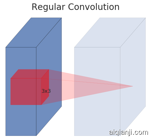
(a) Regular

(b) Separable
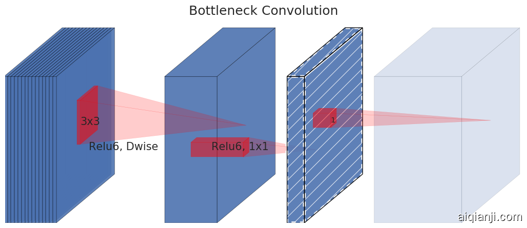
(c) Separable with linear bottleneck
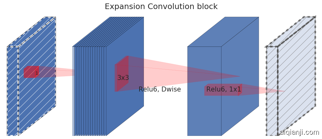
(d) Bottleneck with expansion layer
Figure 2: Evolution of separable convolution blocks. The diagonally hatched texture indicates layers that do not contain non-linearities. The last (lightly colored) layer indicates the beginning of the next block. Note: 1(d) and 1(c) are equivalent blocks when stacked. Best viewed in color.
3.3. 倒置残差
The bottleneck blocks appear similar to residual block where each block contains an input followed by several bottlenecks then followed by expansion [1]. However, inspired by the intuition that the bottlenecks actually contain all the necessary information, while an expansion layer acts merely as an implementation detail that accompanies a non-linear transformation of the tensor, we use shortcuts directly between the bottlenecks. Figure 3 provides a schematic visualization of the difference in the designs. The motivation for inserting shortcuts is similar to that of classical residual connections: we want to improve the ability of a gradient to propagate across multiplier layers. However, the inverted design is considerably more memory efficient (see Section 4 for details), as well as works slightly better in our experiments.
瓶颈块与残差块类似,其中每个块包含一个输入,然后是几个瓶颈,然后是扩展[8]。然而,受直觉的启发,瓶颈实际上包含所有必要的信息,而扩展层只是伴随张量非线性变换的实现细节,我们直接在瓶颈之间使用快捷连接。图3提供了设计差异的示意图。插入快捷连接的动机与经典的残差连接类似:我们想要提高梯度在乘法层之间传播的能力。但是,倒置设计的内存效率要高得多(详见第5节),而且在我们的实验中效果稍好。
Finally, in our network design layers become removable: we can remove a convolutional block and rewire the rest of the network, without any retraining it results in a very modest cost to the accuracy. Similar experimental results were reported in [29]. The crucial difference, however, is that in residual networks the bottleneck layers are treated as low-dimensional supplements to high-dimensional “information” tensors. We refer to Section 6.4 for further details.
最后,在我们的网络设计中,层可以移动:我们可以移除卷积块并重新布线其余的网络,而无需进行任何重新训练,从而导致精度损失非常小。在[ 29 ]中报道了类似的实验结果。但是,关键的区别在于,在残差网络中,瓶颈层被视为对高维“信息”张量的低维补充。有关更多详细信息,请参见第6.4节 。

Figure 3: The difference between residual block [1, 28] and inverted residual. Diagonally hatched layers do not use non-linearities. We use thickness of each block to indicate its relative number of channels. Note how classical residuals connects the layers with high number of channels, whereas the inverted residuals connect the bottlenecks. Best viewed in color.
图3:残差块[8,30]和倒置残差之间的差异。对角阴影线层不使用非线性。我们用每个块的厚度来表明其相对数量的通道。注意经典残差是如何将通道数量较多的层连接起来的,而倒置残差则是连接瓶颈。最好通过颜色看。
Running time and parameter count for bottleneck convolution
The basic implementation structure is illustrated in Table 1. For a block of size h×w, expansion factor t and kernel size k with d′ input channels and d′′ output channels, the total number of multiply add required is h⋅w⋅d′⋅t(d′+k2+d′′). Compared with (1) this expression has an extra term, as indeed we have an extra 1×1 convolution, however the nature of our networks allows us to utilize much smaller input and output dimensions. In Table 3 we compare the needed sizes for each resolution between MobileNetV1, MobileNetV2 and ShuffleNet.
瓶颈卷积的运行时间和参数计数基本实现结构如表1所示。对于大小为$h\times w$的块,扩展因子为$t$,内核大小为$k$,具有$d’$维输入通道和$d’’$维输出通道,所需的乘法加法总数为$h \cdot w \cdot d’ \cdot t(d’ + k^2 + d’’)$。与(1)相比,这个表达式有一个额外项,因为实际上我们有一个额外的1×1卷积,但是我们的网络性质使我们能够利用更小的输入和输出维度。在表3中,我们比较了MobileNetV1,MobileNetV2和ShuffleNet之间每种分辨率所需的尺寸。

Table 1: Bottleneck residual block transforming from k to$k’$ channels, with stride s, and expansion factor t.
表1:瓶颈残差块从$k$转换为$k’$个通道,步长为$s$,扩展系数为$t$。
3.4. 信息流解释 INFORMATION FLOW INTERPRETATION
One interesting property of our architecture is that it provides a natural separation between the input/output domains of the building blocks (bottleneck layers), and the layer transformation – that is a non-linear function that converts input to the output. The former can be seen as the capacity of the network at each layer, whereas the latter as the expressiveness. This is in contrast with traditional convolutional blocks, both regular and separable, where both expressiveness and capacity are tangled together and are functions of the output layer depth.
我们架构的一个有趣特性是它在构建块(瓶颈层)的输入/输出域与层转换之间提供了自然分离——这是一种将输入转换为输出的非线性函数。前者可以看作是网络在每一层的容量,而后者则是表现力。与常规和可分离的传统卷积块相比,其中表现力和容量都缠结在一起并且是输出层深度的函数。
In particular, in our case, when inner layer depth is 0 the underlying convolution is the identity function thanks to the shortcut connection. When the expansion ratio is smaller than 1, this is a classical residual convolutional block [1, 28]. However, for our purposes we show that expansion ratio greater than 1 is the most useful.
特别是在我们的实例中,当内层深度为0时,由于快捷连接,基础卷积是恒等函数。当扩展比率小于1时,这是一个经典的残差卷积块[8,30]。但是,就我们的目的而言,我们表明扩大比率大于1是最有用的。
This interpretation allows us to study the expressiveness of the network separately from its capacity and we believe that further exploration of this separation is warranted to provide a better understanding of the network properties.
这种解释使我们能够独立于其容量研究网络的表现力,并且我们认为需要进一步探索这种分离,以便更好地理解网络性质。
4. 模型架构 MODEL ARCHITECTURE
Now we describe our architecture in detail. As discussed in the previous section the basic building block is a bottleneck depth-separable convolution with residuals. The detailed structure of this block is shown in Table 1. The architecture of MobileNetV2 contains the initial fully convolution layer with 32 filters, followed by 19 residual bottleneck layers described in the Table 2. We use ReLU6 as the non-linearity because of its robustness when used with low-precision computation [26]. We always use kernel size 3×3 as is standard for modern networks, and utilize dropout and batch normalization during training.
现在我们详细描述我们的架构。正如前一节所讨论的那样,基本构件块是一个瓶颈深度可分离的残差卷积。该模块的详细结构如表1所示。MobileNetV2的架构包含具有32个滤波器的初始全卷积层,接着是表2中描述的19个残差瓶颈层。我们使用ReLU6作为非线性,因为用于低精度计算时它的鲁棒性[27]。我们总是使用现代网络中的标准核尺寸3×3,并在训练期间利用丢弃和批归一化。

Table 2: MobileNetV2 : Each line describes a sequence of 1 or more identical (modulo stride) layers, repeated n times. All layers in the same sequence have the same number c of output channels. The first layer of each sequence has a stride s and all others use stride 1. All spatial convolutions use 3×3 kernels. The expansion factor t is always applied to the input size as described in Table 1
表2:MobileNetV2:每行描述一个或多个相同(模步长)层的序列,重复$n$次。同一序列中的所有图层具有相同数量的$c$个输出通道。每个序列的第一层有一个步长$s$,所有其他的都使用长$1$。所有空间卷积使用3×3的核。扩展系数$t$总是应用于输入尺寸,如表1所述。
With the exception of the first layer, we use constant expansion rate throughout the network. In our experiments we find that expansion rates between 5 and 10 result in nearly identical performance curves, with smaller networks being better off with slightly smaller expansion rates and larger networks having slightly better performance with larger expansion rates.
除第一层外,我们在整个网络中使用恒定的扩展率。在我们的实验中,我们发现5到10之间的扩展速率导致几乎相同的性能曲线,较小的网络以较小的扩展速率更好,而较大的网络在较大扩展速率时具有稍微更好的性能。
For all our main experiments we use expansion factor of 6 applied to the size of the input tensor. For example, for a bottleneck layer that takes 64-channel input tensor and produces a tensor with 128 channels, the intermediate expansion layer is then 64⋅6=384 channels.
对于我们所有的主要实验,我们使用扩展因子$6$来应用于输入张量的大小。例如,对于瓶颈层采用$64$通道的输入张量并产生具有$128$通道的张量,中间扩展层则具有$64·6 =384$个通道。
| Size | MobileNetV1 | MobileNetV2 | ShuffleNet |
|---|---|---|---|
| (2x,g=3) | |||
| 112x112 | 1/O(1) | 1/O(1) | 1/O(1) |
| 56x56 | 128/800 | 32/200 | 48/300 |
| 28x28 | 256/400 | 96/150 | 400/600K |
| 14x14 | 512/200 | 160/62 | 800/310 |
| 7x7 | 1024/199 | 320/32 | 1600/156 |
| 1x1 | 1024/2 | 1280/2 | 1600/3 |
| max | 800K | 200K | 600K |
表3:不同架构中需要在每个空间分辨率上实现的最大通道数/内存(以Kb为单位)。我们假设激活使用16位浮点数。对于ShuffleNet,我们使用与MobileNetV1和MobileNetV2的性能相匹配的$2x,g = 3 $。对于MobileNetV2和ShuffleNet的第一层,我们可以采用第5节中描述的技巧来降低内存需求。尽管ShuffleNet在其它地方使用了瓶颈,但由于存在非瓶颈张量之间的快捷连接,因此非瓶颈张量仍然需要实现。
Table 3: The max number of channels/memory (in Kb) that needs to be materialized at each spatial resolution for different architectures. We assume 16-bit floats for activations. For ShuffleNet, we use 2x,g=3 that matches the performance of MobileNetV1 and MobileNetV2. For the first layer of MobileNetV2 and ShuffleNet we can employ the trick described in Section 4 to reduce memory requirement. Even though ShuffleNet employs bottlenecks elsewhere, the non-bottleneck tensors still need to be materialized due to the presence of shortcuts between non-bottleneck te
Trade-off hyper parameters
As in [26] we tailor our architecture to different performance points, by using the input image resolution and width multiplier as tunable hyper parameters, that can be adjusted depending on desired accuracy/performance trade-offs. Our primary network (width multiplier 1, 224×224), has a computational cost of 300 million multiply-adds and uses 3.4 million parameters. We explore the performance trade offs, for input resolutions from 96 to 224, and width multipliers of 0.35 to 1.4. The network computational cost ranges from 7 multiply adds to 585M MAdds, while the model size vary between 1.7M and 6.9M parameters.
One minor implementation difference, with [26] is that for multipliers less than one, we apply width multiplier to all layers except the very last convolutional layer. This improves performance for smaller models.
和[27]一样,我们通过使用输入图像分辨率和宽度倍数作为可调超参数来调整我们的架构以适应不同的性能点,可以根据所需的精度/性能权衡来调整。我们的主要网络(宽度乘数1,224×224)的计算成本为3亿次乘法,并使用了340万个参数。我们研究了性能权衡,输入分辨率从96到224,宽度乘数从0.35到1.4。网络计算成本范围从7次乘法增加到585M MAdds,而模型大小在1.7M个参数和6.9M个参数之间变化。
一个较小的实现差异,[27]是对于小于1的乘数,我们将宽度乘数应用于除最后一个卷积层以外的所有层。这可以提高更小模型的性能。
5. 实现说明 IMPLEMENTATION NOTES
 (a) NasNet[22]
 (b) MobileNet[26]
 (c) ShuffleNet [19]
 (d) Mobilenet V2
Figure 4: Comparison of convolutional blocks for different architectures. ShuffleNet uses Group Convolutions [19] and shuffling, it also uses conventional residual approach where inner blocks are narrower than output. ShuffleNet and NasNet illustrations are from respective papers.
5.1. 内存有效推断 MEMORY EFFICIENT INFERENCE
The inverted residual bottleneck layers allow a particularly memory efficient implementation which is very important for mobile applications. A standard efficient implementation of inference that uses for instance TensorFlow[30] or Caffe [31], builds a directed acyclic compute hypergraph G, consisting of edges representing the operations and nodes representing tensors of intermediate computation. The computation is scheduled in order to minimize the total number of tensors that needs to be stored in memory. In the most general case, it searches over all plausible computation orders Σ(G) and picks the one that minimizes
倒置的残差颈层允许特定地内存有效的实现,这对于移动应用非常重要。使用TensorFlow[31]或Caffe[32]等标准高效的推断实现,构建了一个有向无环计算超图$G$,由表示操作的边和代表中间计算张量的节点组成。预定计算是为了最小化需要存储在内存中的张量总数。在最一般的情况下,它会搜索所有合理的计算顺序$\Sigma (G)$,并选择最小化
$$ M(G) = \min_{\pi\in \Sigma(G)} \max_{i \in 1..n} \left[\sum_{A \in R(i, \pi, G)} |A|\right] + \text{size}(\pi_i) $$
where R(i,π,G) is the list of intermediate tensors that are connected to any of πi…πn nodes, |A| represents the size of the tensor A and size(i) is the total amount of memory needed for internal storage during operation i.
For graphs that have only trivial parallel structure (such as residual connection), there is only one non-trivial feasible computation order, and thus the total amount and a bound on the memory needed for inference on compute graph G can be simplified:
。其中$R(i, \pi, G)$是连接到任何$\pi_{i}\dots \pi_{n}$节点的中间张量列表,$|A|$表示张量$A$的大小,$size(i)$是操作$i$期间内部存储所需的总内存量。
对于仅具有平凡并行结构(例如残差连接)的图,只有一个非平凡的可行计算顺序,因此可以简化计算图$G$推断所需的内存总量和界限:
$$
M(G) = \max_{op \in G} \left[\sum_{A \in \text{op}{inp}} |A| + \sum{B \in \text{op}_{out}} |B| + |op|\right] \tag {2}
$$
Or to restate, the amount of memory is simply the maximum total size of combined inputs and outputs across all operations. In what follows we show that if we treat a bottleneck residual block as a single operation (and treat inner convolution as a disposable tensor), the total amount of memory would be dominated by the size of bottleneck tensors, rather than the size of tensors that are internal to bottleneck (and much larger).
或者重申,内存量只是在所有操作中组合输入和输出的最大总大小。在下文中我们将展示如果我们将瓶颈残差块视为单一操作(并将内部卷积视为一次性张量),则总内存量将由瓶颈张量的大小决定,而不是瓶颈的内部张量的大小(更大)。
Bottleneck Residual Block
A bottleneck block operator F(x) shown in Figure 2(b) can be expressed as a composition of three operators F(x)=[A∘N∘B]x, where A is a linear transformation A:Rs×s×k→Rs×s×n, N is a non-linear per-channel transformation: N:Rs×s×n→Rs′×s′×n, and B is again a linear transformation to the output domain: B:Rs′×s′×n→Rs′×s′×k′.
For our networks N=ReLU6∘dwise∘ReLU6, but the results apply to any per-channel transformation. Suppose the size of the input domain is |x| and the size of the output domain is |y|, then the memory required to compute F(X) can be as low as $|s^2 k| + |s’^2 k’| + O(\max(s^2, s’^2))$.
瓶颈残差块 图3b中所示的$\mathcal{F}(x)$可以表示为三个运算符的组合$\mathcal{F}(x) = [A \circ \mathcal{N} \circ B] x$,其中$A$是线性变换$A:\mathcal{R}^{s \times s \times k} \rightarrow \mathcal{R}^{s \times s \times n}$,$\mathcal{N}$是一个非线性的每个通道的转换:$\mathcal{N}: \mathcal{R}^{s \times s \times n} \rightarrow \mathcal{R}^{s’ \times s’ \times n}$,$B$是输出域的线性转换:$B: \mathcal{R}^{s’ \times s’ \times n} \rightarrow \mathcal{R}^{s’ \times s’ \times k’}$。
对于我们的网络$\mathcal{N} = ReLU6 \circ dwise \circ ReLU6$,但结果适用于任何的按通道转换。假设输入域的大小是$|x|$并且输出域的大小是$|y|$,那么计算$F(X)$所需的内存可以低至$|s^2 k| + |s’^2 k’| + O(\max(s^2, s’^2))$。
The algorithm is based on the fact that the inner tensor I can be represented as concatenation of t tensors, of size n/t each and our function can then be represented as
该算法基于以下事实:内部张量$\cal I$可以表示为$t$张量的连接,每个大小为$n/t$,则我们的函数可以表示为
$$
\mathcal{F}(x) = \sum_{i=1}^t (A_i \circ N \circ B_i)(x)
$$
by accumulating the sum, we only require one intermediate block of size n/t to be kept in memory at all times. Using n=t we end up having to keep only a single channel of the intermediate representation at all times. The two constraints that enabled us to use this trick is (a) the fact that the inner transformation (which includes non-linearity and depthwise) is per-channel, and (b) the consecutive non-per-channel operators have significant ratio of the input size to the output. For most of the traditional neural networks, such trick would not produce a significant improvement.
通过累加和,我们只需要将一个大小为$n/t$的中间块始终保留在内存中。使用$n=t$,我们最终只需要保留中间表示的单个通道。使我们能够使用这一技巧的两个约束是(a)内部变换(包括非线性和深度)是每个通道的事实,以及(b)连续的非按通道运算符具有显著的输入输出大小比。对于大多数传统的神经网络,这种技巧不会产生显著的改善。
We note that, the number of multiply-adds operators needed to compute F(X) using t-way split is independent of t, however in existing implementations we find that replacing one matrix multiplication with several smaller ones hurts runtime performance due to increased cache misses. We find that this approach is the most helpful to be used with t being a small constant between 2 and 5. It significantly reduces the memory requirement, but still allows one to utilize most of the efficiencies gained by using highly optimized matrix multiplication and convolution operators provided by deep learning frameworks. It remains to be seen if special framework level optimization may lead to further runtime improvements.
我们注意到,使用$t$路分割计算$F(X)$所需的乘加运算符的数目是独立于$t$的,但在现有实现中,我们发现由于增加的缓存未命中,用几个较小的矩阵乘法替换一个矩阵乘法会很损坏运行时的性能 。我们发现这种方法最有用,$t$是$2$和$5$之间的一个小常数。它显著降低了内存需求,但仍然可以利用深度学习框架提供的高度优化的矩阵乘法和卷积算子来获得的大部分效率。如果特殊的框架级优化可能导致进一步的运行时改进,这个方法还有待观察。
6. 实验 EXPERIMENTS
6.1. ImageNet分类 IMAGENET CLASSIFICATION
Training setup
We train our models using TensorFlow[30]. We use the standard RMSPropOptimizer with both decay and momentum set to 0.9. We use batch normalization after every layer, and the standard weight decay is set to 0.00004. Following MobileNetV1[26] setup we use initial learning rate of 0.045, and learning rate decay rate of 0.98 per epoch. We use 16 GPU asynchronous workers, and a batch size of 96.
Results
We compare our networks against MobileNetV1, ShuffleNet and NASNet-A models. The statistics of a few selected models is shown in Table 4 with the full performance graph shown in Figure 5.
训练设置我们使用TensorFlow[31]训练我们的模型。我们使用标准的RMSPropOptimizer,将衰减和动量都设置为0.9。我们在每层之后使用批标准化,并将标准权重衰减设置为0.00004。遵循MobileNetV1 [27]的设置,我们使用初始学习率为0.045,学习率的衰减比率为每个迭代周期衰减0.98。我们使用16个GPU异步,批大小为96。
结果我们将我们的网络与MobileNetV1,ShuffleNet和NASNet-A模型进行了比较。表4列出了一些选定模型的统计数据,完整的性能图如图5所示。
| Network | Top 1 | Params | MAdds | CPU |
|---|---|---|---|---|
| MobileNetV1 | 70.6 | 4.2M | 575M | 123ms |
| ShuffleNet (1.5) | 69.0 | 2.9M | 292M | - |
| ShuffleNet (x2) | 70.9 | 4.4M | 524M | - |
| NasNet-A | 74.0 | 5.3M | 564M | 192ms |
| MobileNetV2 | 71.7 | 3.4M | 300M | 80ms |
| MobileNetV2 (1.4) | 74.7 | 6.9M | 585M | 149ms |
Table 4: Performance on ImageNet, comparison for different networks. As is common practice for ops, we count the total number of Multiply-Adds. In the last column we report running time in milliseconds (ms) for a single large core of the Google Pixel 1 phone (using TF-Lite). We do not report ShuffleNet numbers as the framework does not yet support efficient group convolutions.
表4:比较不同网络在ImageNet上的性能。正如ops的常见做法一样,我们计算Multiply-Adds的总数。在最后一列中,我们报告了Google Pixel 1手机上的一个大型核心(使用TF-Lite)的运行时间,以毫秒(ms)为单位。我们不报告ShuffleNet的数字,因为高效的群组卷积和混排尚未支持。

图5:MobileNetV2与MobileNetV1,ShuffleNet,NAS的性能曲线。对于我们的网络,我们对所有分辨率使用乘数0.35,0.5,0.75,1.0,对于分辨率为224,我们使用乘数1.4。
6.2. 目标检测 OBJECT DETECTION
We evaluate and compare the performance of MobileNetV2 and MobileNetV1 as feature extractors [32] for object detection with a modified version of the Single Shot Detector (SSD) [33] on COCO dataset [3]. We also compare to YOLOv2 [34] and original SSD (with VGG-16 [6] as base network) as baselines. We do not compare performance with other architectures such as Faster-RCNN [35] and RFCN [36] since our focus is on mobile/real-time models.
SSDLite: In this paper, we introduce a mobile friendly variant of regular SSD. We replace all the regular convolutions with separable convolutions (depthwise followed by 1×1 projection) in SSD prediction layers. This design is in line with the overall design of MobileNets and is seen to be much more computationally efficient. We call this modified version SSDLite. Compared to regular SSD, SSDLite dramatically reduces both parameter count and computational cost as shown in Table 5.
我们评估和比较了MobileNetV2和MobileNetV1的性能,MobileNetV1使用COCO数据集[2]上Single Shot Detector(SSD)[34]的修改版本作为目标检测的特征提取器[33]。我们还将YOLOv2[35]和原始SSD(以VGG-16[6]为基础网络)作为基准进行比较。由于我们专注于移动/实时模型,因此我们不会比较Faster-RCNN[36]和RFCN[37]等其它架构的性能。
SSDLite 在本文中,我们将介绍常规SSD的移动友好型变种。我们在SSD预测层中用可分离卷积(深度方向后接$1\times 1$投影)替换所有常规卷积。这种设计符合MobileNets的整体设计,并且在计算上效率更高。我们称之为修改版本的SSDLite。与常规SSD相比,SSDLite显著降低了参数计数和计算成本,如表5所示。
| Params | MAdds | |
|---|---|---|
| SSD[33] | 14.8M | 1.25B |
| SSDLite | 2.1M | 0.35B |
Table 5: Comparison of the size and the computational cost between SSD and SSDLite configured with MobileNetV2 and making predictions for 80 classes.
表5:使用MobileNetV2配置的SSD和SSDLite之间的大小和计算成本以及对80个类进行预测的比较。
For MobileNetV1, we follow the setup in [32]. For MobileNetV2, the first layer of SSDLite is attached to the expansion of layer 15 (with output stride of 16). The second and the rest of SSDLite layers are attached on top of the last layer (with output stride of 32). This setup is consistent with MobileNetV1 as the first and second layers are attached to the feature map of the same output strides.
Both MobileNet models are trained and evaluated with Open Source TensorFlow Object Detection API [37]. The input resolution of both models is 320×320. We benchmark and compare both mAP (COCO challenge metrics), number of parameters and number of Multiply-Adds. The results are shown in Table 6. MobileNetV2 SSDLite is not only the most efficient model, but also the most accurate of the three. Notably, MobileNetV2 SSDLite is 20× more efficient and 10× smaller while still outperforms YOLOv2 on COCO dataset.
对于MobileNetV1,我们按照[33]中的设置进行。对于MobileNetV2,SSDLite的第一层被附加到层15的扩展(输出步长为16)。SSDLite层的第二层和其余层连接在最后一层的顶部(输出步长为32)。此设置与MobileNetV1一致,因为所有层都附加到相同输出步长的特征图上。
MobileNet模型都经过了开源TensorFlow目标检测API的训练和评估[38]。 两个模型的输入分辨率为$320 \times 320$。我们进行了基准测试并比较了mAP(COCO挑战度量标准),参数数量和Multiply-Adds数量。结果如表6所示。MobileNetV2 SSDLite不仅是最高效的模型,而且也是三者中最准确的模型。值得注意的是,MobileNetV2 SSDLite效率高20倍,模型要小10倍,但仍优于COCO数据集上的YOLOv2。
| Network | mAP | Params | MAdd | CPU |
|---|---|---|---|---|
| SSD300[33] | 23.2 | 36.1M | 35.2B | - |
| SSD512[33] | 26.8 | 36.1M | 99.5B | - |
| YOLOv2[34] | 21.6 | 50.7M | 17.5B | - |
| MNet V1 + SSDLite | 22.2 | 5.1M | 1.3B | 270ms |
| MNet V2 + SSDLite | 22.1 | 4.3M | 0.8B | 200ms |
Table 6: Performance comparison of MobileNetV2 + SSDLite and other realtime detectors on the COCO dataset object detection task. MobileNetV2 + SSDLite achieves competitive accuracy with significantly fewer parameters and smaller computational complexity. All models are trained on trainval35k and evaluated on test-dev. SSD/YOLOv2 numbers are from [34]. The running time is reported for the large core of the Google Pixel 1 phone, using an internal version of the TF-Lite engine.
表6:MobileNetV2+SSDLite和其他实时检测器在COCO数据集目标检测任务中的性能比较。MobileNetV2+SSDLite以更少的参数和更小的计算复杂性实现了具有竞争力的精度。所有模型都在trainval35k上进行训练,并在test-dev上进行评估。SSD/YOLOv2的数字来自于[35]。使用内部版本的TF-Lite引擎,报告了在Google Pixel 1手机的大型核心上的运行时间。
6.3. 语义分割 SEMANTIC SEGMENTATION
In this section, we compare MobileNetV1 and MobileNetV2 models used as feature extractors with DeepLabv3 [38] for the task of mobile semantic segmentation. DeepLabv3 adopts atrous convolution [39, 40, 41], a powerful tool to explicitly control the resolution of computed feature maps, and builds five parallel heads including (a) Atrous Spatial Pyramid Pooling module (ASPP) [42] containing three 3×3 convolutions with different atrous rates, (b) 1×1 convolution head, and (c) Image-level features [43]. We denote by output_stride the ratio of input image spatial resolution to final output resolution, which is controlled by applying the atrous convolution properly. For semantic segmentation, we usually employ \emphoutput_stride=16 or 8 for denser feature maps. We conduct the experiments on the PASCAL VOC 2012 dataset [4], with extra annotated images from [44] and evaluation metric mIOU.
在本节中,我们使用MobileNetV1和MobileNetV2模型作为特征提取器与DeepLabv3[39]在移动语义分割任务上进行比较。DeepLabv3采用了空洞卷积[40,41,42],这是一种显式控制计算特征映射分辨率的强大工具,并构建了五个平行头部,包括(a)包含三个具有不同空洞率的$3 \times 3$卷积的Atrous Spatial Pyramid Pooling模块(ASPP)[43],(b)$1 \times 1$卷积头部,以及(c)图像级特征[44]。我们用输出步长来表示输入图像空间分辨率与最终输出分辨率的比值,该分辨率通过适当地应用空洞卷积来控制。对于语义分割,我们通常使用输出$stride = 16$或$8$来获取更密集的特征映射。我们在PASCAL VOC 2012数据集[3]上进行了实验,使用[45]中的额外标注图像和评估指标mIOU。
To build a mobile model, we experimented with three design variations: (1) different feature extractors, (2) simplifying the DeepLabv3 heads for faster computation, and (3) different inference strategies for boosting the performance. Our results are summarized in Table 7. We have observed that: (a) the inference strategies, including multi-scale inputs and adding left-right flipped images, significantly increase the MAdds and thus are not suitable for on-device applications, (b) using \emphoutput_stride=16 is more efficient than \emphoutput_stride=8, (c) MobileNetV1 is already a powerful feature extractor and only requires about 4.9−5.7 times fewer MAdds than ResNet-101 [1] (*e.g*., mIOU: 78.56 *vs* 82.70, and MAdds: 941.9B *vs* 4870.6B), (d) it is more efficient to build DeepLabv3 heads on top of the second last feature map of MobileNetV2 than on the original last-layer feature map, since the second to last feature map contains 320 channels instead of 1280, and by doing so, we attain similar performance, but require about 2.5 times fewer operations than the MobileNetV1 counterparts, and (e) DeepLabv3 heads are computationally expensive and removing the ASPP module significantly reduces the MAdds with only a slight performance degradation. In the end of the Table 7, we identify a potential candidate for on-device applications (in bold face), which attains 75.32% mIOU and only requires 2.75B MAdds.
为了构建移动模型,我们尝试了三种设计变体:(1)不同的特征提取器,(2)简化DeepLabv3头部以加快计算速度,以及(3)提高性能的不同推断策略。我们的结果总结在表7中。我们已经观察到:(a)包括多尺度输入和添加左右翻转图像的推断策略显著增加了MAdds,因此不适合于在设备上应用,(b)使用输出步长16比使用输出步长8更有效率,(c)MobileNetV1已经是一个强大的特征提取器,并且只需要比ResNet-101少约4.9-5.7倍的MAdd[8](例如,mIOU:78.56与82.70和MAdds:941.9B vs 4870.6B),(d)在MobileNetV2的倒数第二个特征映射的顶部构建DeepLabv3头部比在原始的最后一个特征映射上更高效,因为倒数第二个特征映射包含320个通道而不是1280个通道,这样我们就可以达到类似的性能,但是要比MobileNetV1的通道少2.5倍,(e)DeepLabv3头部的计算成本很高,移除ASPP模块会显著减少MAdd并且只会稍微降低性能。在表7末尾,我们鉴定了一个设备上的潜在候选应用(粗体),该应用可以达到$75.32%$mIOU并且只需要2.75B MAdds。
| Network | OS | ASPP | MF | mIOU | Params | MAdds |
|---|---|---|---|---|---|---|
| MNet V1 | 16 | ✓ | 75.29 | 11.15M | 14.25B | |
| 8 | ✓ | ✓ | 78.56 | 11.15M | 941.9B | |
| MNet V2* | 16 | ✓ | 75.70 | 4.52M | 5.8B | |
| 8 | ✓ | ✓ | 78.42 | 4.52M | 387B | |
| MNet V2* | 16 | 75.32 | 2.11M | 2.75B | ||
| 8 | ✓ | 77.33 | 2.11M | 152.6B | ||
| ResNet-101 | 16 | ✓ | 80.49 | 58.16M | 81.0B | |
| 8 | ✓ | ✓ | 82.70 | 58.16M | 4870.6B |
Table 7: MobileNet + DeepLabv3 inference strategy on the PASCAL VOC 2012 validation set. MNet V2*: Second last feature map is used for DeepLabv3 heads, which includes (1) Atrous Spatial Pyramid Pooling (ASPP) module, and (2) 1×1 convolution as well as image-pooling feature. OS: output_stride that controls the output resolution of the segmentation map. MF: Multi-scale and left-right flipped inputs during test. All of the models have been pretrained on COCO. The potential candidate for on-device applications is shown in bold face. PASCAL images have dimension 512×512 and atrous convolution allows us to control output feature resolution without increasing the number of parameters.
表7:PASCAL VOC 2012验证集上的MobileNet+DeepLabv3推断策略。MNet V2*:用于DeepLabv3头部的倒数第二个特征映射,其中包括(1)Atrous Spatial Pyramid Pooling(ASPP)模块和(2)$1\times 1$卷积以及图像池化功能。OS:控制分割映射输出分辨率的输出步长。MF:测试期间多尺度和左右翻转输入。所有的模型都在COCO上进行预训练。设备上的潜在候选应用以粗体显示。PASCAL图像的尺寸为$ 512 \ times 512 $,而空洞卷积使得我们可以在不增加参数数量的情况下控制输出特征分辨率。
6.4. 消融研究 ABLATION STUDY
Inverted residual connections. The importance of residual connection has been studied extensively [1, 28, 45]. The new result reported in this paper is that the shortcut connecting bottleneck perform better than shortcuts connecting the expanded layers (see Figure 5(b) for comparison).
Importance of linear bottlenecks. Theoretically, the linear bottleneck models are strictly less powerful than models with non-linearities, because the activations can always operate in linear regime with appropriate changes to biases and scaling. However our experiments shown in Figure 5(a) indicate that linear bottlenecks improve performance, providing a strong support for the hypothesis that a non-linearity operator is not beneficial in the low-dimensional space of a bottleneck.
倒置残差连接。残差连接的重要性已被广泛研究[8,30,46]。本文报告的新结果是连接瓶颈的快捷连接性能优于连接扩展层的的快捷连接(请参见图6b以供比较)。

Figure 6: The impact of non-linearities and various types of shortcut (residual) connections.
图6:非线性和各种快捷(残差)连接的影响。
线性瓶颈的重要性。线性瓶颈模型的严格来说比非线性模型要弱一些,因为激活总是可以在线性状态下进行,并对偏差和缩放进行适当的修改。然而,我们在图6a中展示的实验表明,线性瓶颈改善了性能,为非线性破坏低维空间中的信息提供了支持。
7. 总结及将来工作 CONCLUSIONS AND FUTURE WORK
We described a new network architecture that allowed us to build a family of efficient mobile models that improves the state of the art at a wide range of performance points. Our basic building unit, has several properties that make it particularly suitable for mobile applications. It allows very memory-efficient inference and can utilize standard operations present in all neural frameworks.
For the ImageNet dataset, our architecture works for models ranging from 10 Million Mult-Adds to 580 Million Mult-Adds improving on the state of the art. Additionally, the architectures are dramatically simpler than the previous state of the art based on automatic network search.
For object detection task, our network outperforms state-of-art realtime detectors on COCO dataset both in terms of accuracy and model complexity. Notably, our architecture combined with the SSDLite detection module is 20× less computation and 10× less parameters than YOLOv2.
On the theoretical side: the proposed convolutional block has a unique property that allows to separate the network expressivity (encoded by expansion layers) from its capacity (encoded by bottleneck inputs). Exploring this is an important direction for future research.
我们描述了一个非常简单的网络架构,使我们能够构建一系列高效的移动模型。我们的基本构建单元具有多种特性,使其特别适用于移动应用。它允许非常有效的内存推断,并依赖利用所有神经框架中的标准操作。
对于ImageNet数据集,我们的架构改善了许多性能点的最新技术水平。对于目标检测任务,我们的网络在精度和模型复杂度方面都优于COCO数据集上的最新实时检测器。值得注意的是,我们的架构与SSDLite检测模块相比,计算量少20倍,参数比YOLOv2少10倍。
理论上:所提出的卷积块具有独特的属性,允许将网络表现力(由扩展层编码)与其容量(由瓶颈输入编码)分开。探索这个是未来研究的重要方向。
致谢 Acknowledgments
我们要感谢Matt Streeter和Sergey Ioffe的有益反馈和讨论。
We would like to thank Matt Streeter and Sergey Ioffe for their helpful feedback and discussion.
References
[1] Olga Russakovsky, Jia Deng, Hao Su, Jonathan Krause, Sanjeev Satheesh, Sean Ma, Zhiheng Huang, Andrej Karpathy, Aditya Khosla, Michael Bernstein, Alexander C. Berg, and Li Fei-Fei. Imagenet large scale visual recognition challenge. Int. J. Comput. Vision, 115(3):211–252, December 2015.
[2] Tsung-Yi Lin, Michael Maire, Serge Belongie, James Hays, Pietro Perona, Deva Ramanan, Piotr Dollár, and C Lawrence Zitnick. Microsoft COCO: Common objects in context. In ECCV, 2014.
[3] Mark Everingham, S. M. Ali Eslami, Luc Van Gool, Christopher K. I. Williams, John Winn, and Andrew Zisserma. The pascal visual object classes challenge a retrospective. IJCV, 2014.
[4] Mobilenetv2 source code. Available from https://github.com/tensorflow/ models/tree/master/research/slim/nets/mobilenet.
[5] Alex Krizhevsky, Ilya Sutskever, and Geoffrey E. Hinton. Imagenet classification with deep convolutional neural networks. In Bartlett et al. [48], pages 1106–1114.
[6] Karen Simonyan and Andrew Zisserman. Very deep convolutional networks for large-scale image recognition. CoRR, abs/1409.1556, 2014.
[7] Christian Szegedy, Wei Liu, Yangqing Jia, Pierre Sermanet, Scott E. Reed, Dragomir Anguelov, Dumitru Erhan, Vincent Vanhoucke, and Andrew Rabinovich. Going deeper with convolutions. In IEEE Conference on Computer Vision and Pattern Recognition, CVPR 2015, Boston, MA, USA, June 7-12, 2015, pages 1–9. IEEE Computer Society, 2015.
[8] Kaiming He, Xiangyu Zhang, Shaoqing Ren, and Jian Sun. Deep residual learning for image recognition. CoRR, abs/1512.03385, 2015.
[9] James Bergstra and Yoshua Bengio. Random search for hyper-parameter optimization. Journal of Machine Learning Research, 13:281–305, 2012.
[10] Jasper Snoek, Hugo Larochelle, and Ryan P. Adams. Practical bayesian optimization of machine learning algorithms. In Bartlett et al. [48], pages 2960–2968.
[11] Jasper Snoek, Oren Rippel, Kevin Swersky, Ryan Kiros, Nadathur Satish, Narayanan Sundaram, Md. Mostofa Ali Patwary, Prabhat, and Ryan P. Adams. Scalable bayesian optimization using deep neural networks. In Francis R. Bach and David M. Blei, editors, Proceedings of the 32nd International Conference on Machine Learning, ICML 2015, Lille, France, 6-11 July 2015, volume 37 of JMLR Workshop and Conference Proceedings, pages 2171–2180. JMLR.org, 2015.
[12] Babak Hassibi and David G. Stork. Second order derivatives for network pruning: Optimal brain surgeon. In Stephen Jose Hanson, Jack D. Cowan, and C. Lee Giles, editors, Advances in Neural Information Processing Systems 5, [NIPS Conference, Denver, Colorado, USA, November 30 - December 3, 1992], pages 164–171. Morgan Kaufmann, 1992.
[13] Yann LeCun, John S. Denker, and Sara A. Solla. Optimal brain damage. In David S. Touretzky, editor, Advances in Neural Information Processing Systems 2, [NIPS Conference, Denver, Colorado, USA, November 27-30, 1989], pages 598–605. Morgan Kaufmann, 1989.
[14] Song Han, Jeff Pool, John Tran, and William J. Dally. Learning both weights and connections for efficient neural network. In Corinna Cortes, Neil D. Lawrence, Daniel D. Lee, Masashi Sugiyama, and Roman Garnett, editors, Advances in Neural Information Processing Systems 28: Annual Conference on Neural Information Processing Systems 2015, December 7-12, 2015, Montreal, Quebec, Canada, pages 1135–1143, 2015.
[15] Song Han, Jeff Pool, Sharan Narang, Huizi Mao, Shijian Tang, Erich Elsen, Bryan Catanzaro, John Tran, and William J. Dally. DSD: regularizing deep neural networks with dense-sparse-dense training flow. CoRR, abs/1607.04381, 2016.
[16] Yiwen Guo, Anbang Yao, and Yurong Chen. Dynamic network surgery for efficient dnns. In Daniel D. Lee, Masashi Sugiyama, Ulrike von Luxburg, Isabelle Guyon, and Roman Garnett, editors, Advances in Neural Information Processing Systems 29: Annual Conference on Neural Information Processing Systems 2016, December 5-10, 2016, Barcelona, Spain, pages 1379–1387, 2016.
[17] Hao Li, Asim Kadav, Igor Durdanovic, Hanan Samet, and Hans Peter Graf. Pruning filters for efficient convnets. CoRR, abs/1608.08710, 2016.
[18] Karim Ahmed and Lorenzo Torresani. Connectivity learning in multi-branch networks. CoRR, abs/1709.09582, 2017.
[19] Tom Veniat and Ludovic Denoyer. Learning time-efficient deep architectures with budgeted super networks. CoRR, abs/1706.00046, 2017.
[20] Xiangyu Zhang, Xinyu Zhou, Mengxiao Lin, and Jian Sun. Shufflenet: An extremely efficient convolutional neural network for mobile devices. CoRR, abs/1707.01083, 2017.
[21] Soravit Changpinyo, Mark Sandler, and Andrey Zhmoginov. The power of sparsity in convolutional neural networks. CoRR, abs/1702.06257, 2017.
[22] Min Wang, Baoyuan Liu, and Hassan Foroosh. Design of efficient convolutional layers using single intra-channel convolution, topological subdivisioning and spatial ”bottleneck” structure. CoRR, abs/1608.04337, 2016.
[23] Barret Zoph, Vijay Vasudevan, Jonathon Shlens, and Quoc V. Le. Learning transferable architectures for scalable image recognition. CoRR, abs/1707.07012, 2017.
[24] Lingxi Xie and Alan L. Yuille. Genetic CNN. CoRR, abs/1703.01513, 2017.
[25] Esteban Real, Sherry Moore, Andrew Selle, Saurabh Saxena, Yutaka Leon Suematsu, Jie Tan, Quoc V. Le, and Alexey Kurakin. Large-scale evolution of image classifiers. In Doina Precup and Yee Whye Teh, editors, Proceedings of the 34th International Conference on Machine Learning, ICML 2017, Sydney, NSW, Australia, 6-11 August 2017, volume 70 of Proceedings of Machine Learning Research, pages 2902–2911. PMLR, 2017.
[26] Barret Zoph and Quoc V. Le. Neural architecture search with reinforcement learning. CoRR, abs/1611.01578, 2016.
[27] Andrew G. Howard, Menglong Zhu, Bo Chen, Dmitry Kalenichenko, Weijun Wang, Tobias Weyand, Marco Andreetto, and Hartwig Adam.
Mobilenets: Efficient convolutional neural networks for mobile vision applications. CoRR, abs/1704.04861, 2017.
[28] Francois Chollet. Xception: Deep learning with depthwise separable convolutions. In The IEEE Conference on Computer Vision and Pattern Recognition (CVPR), July 2017.
[29] Dongyoon Han, Jiwhan Kim, and Junmo Kim. Deep pyramidal residual networks. CoRR, abs/1610.02915, 2016.
[30] Saining Xie, Ross B. Girshick, Piotr Dolla ́r, Zhuowen Tu, and Kaiming He. Aggregated residual transformations for deep neural networks. CoRR, abs/1611.05431, 2016.
[31] Martın Abadi, Ashish Agarwal, Paul Barham, Eugene Brevdo, Zhifeng Chen, Craig Citro, Greg S. Corrado, Andy Davis, Jeffrey Dean, Matthieu Devin, Sanjay Ghemawat, Ian Goodfellow, Andrew Harp, Geoffrey Irving, Michael Isard, Yangqing Jia, Rafal Jozefowicz, Lukasz Kaiser, Manjunath Kudlur, Josh Levenberg, Dan Mané, Rajat Monga, Sherry Moore, Derek Murray, Chris Olah, Mike Schuster, Jonathon Shlens, Benoit Steiner, Ilya Sutskever, Kunal Talwar, Paul Tucker, Vincent Vanhoucke, Vijay Vasudevan, Fernanda Viégas, Oriol Vinyals, Pete Warden, Martin Wattenberg, Martin Wicke, Yuan Yu, and Xiaoqiang Zheng. TensorFlow: Large-scale machine learning on heterogeneous systems, 2015. Software available from tensorflow.org.
[32] Yangqing Jia, Evan Shelhamer, Jeff Donahue, Sergey Karayev, Jonathan Long, Ross Girshick, Sergio Guadarrama, and Trevor Darrell. Caffe: Convolutional architecture for fast feature embed- ding. arXiv preprint arXiv:1408.5093, 2014.
[33] Jonathan Huang, Vivek Rathod, Chen Sun, Men- glong Zhu, Anoop Korattikara, Alireza Fathi, Ian Fischer, Zbigniew Wojna, Yang Song, Sergio Guadarrama, et al. Speed/accuracy trade-offs for modern convolutional object detectors. In CVPR, 2017.
[34] Wei Liu, Dragomir Anguelov, Dumitru Erhan, Christian Szegedy, Scott Reed, Cheng-Yang Fu, and Alexander C Berg. Ssd: Single shot multibox detector. In ECCV, 2016.
[35] Joseph Redmon and Ali Farhadi. Yolo9000: Better, faster, stronger. arXiv preprint arXiv:1612.08242, 2016.
[36] Shaoqing Ren, Kaiming He, Ross Girshick, and Jian Sun. Faster r-cnn: Towards real-time object detection with region proposal networks. In Advances in neural information processing systems, pages 91–99, 2015.
[37] Jifeng Dai, Yi Li, Kaiming He, and Jian Sun. R-fcn: Object detection via region-based fully convolutional networks. In Advances in neural information processing systems, pages 379–387, 2016.
[38] Jonathan Huang, Vivek Rathod, Derek Chow, Chen Sun, and Menglong Zhu. Tensorflow object detection api, 2017.
[39] Liang-Chieh Chen, George Papandreou, Florian Schroff, and Hartwig Adam. Rethinking atrous convolution for semantic image segmentation. CoRR, abs/1706.05587, 2017.
[40] Matthias Holschneider, Richard Kronland-Martinet, Jean Morlet, and Ph Tchamitchian. A real-time algorithm for signal analysis with the help of the wavelet transform. In Wavelets: Time-Frequency Methods and Phase Space, pages 289–297. 1989.
[41] Pierre Sermanet, David Eigen, Xiang Zhang, Michaël Mathieu, Rob Fergus, and Yann LeCun. Overfeat: Integrated recognition, localization and detection using convolutional networks. arXiv:1312.6229, 2013.
[42] George Papandreou,Iasonas Kokkinos, and Pierre Andre Savalle. Modeling local and global deformations in deep learning: Epitomic convolution, multiple instance learning, and sliding window detection. In CVPR, 2015.
[43] Liang-Chieh Chen, George Papandreou, Iasonas Kokkinos, Kevin Murphy, and Alan L Yuille. Deeplab: Semantic image segmentation with deep convolutional nets, atrous convolution, and fully connected crfs. TPAMI, 2017.
[44] Wei Liu, Andrew Rabinovich, and Alexander C. Berg. Parsenet: Looking wider to see better. CoRR, abs/1506.04579, 2015.
[45] Bharath Hariharan, Pablo Arbeláez, Lubomir Bourdev, Subhransu Maji, and Jitendra Malik. Semantic contours from inverse detectors. In ICCV, 2011.
[46] Christian Szegedy, Sergey Ioffe, and Vincent Vanhoucke. Inception-v4, inception-resnet and the impact of residual connections on learning. CoRR, abs/1602.07261, 2016.
[47] Guido Montúfar, Razvan Pascanu, Kyunghyun Cho, and Yoshua Bengio. On the number of linear regions of deep neural networks. In Proceedings of the 27th International Conference on Neural Information Processing Systems, NIPS’14, pages 2924–2932, Cambridge, MA, USA, 2014. MIT Press.
[48] Peter L. Bartlett, Fernando C. N. Pereira, Christopher J. C. Burges, Léon Bottou, and Kilian Q. Weinberger, editors. Advances in Neural Information Processing Systems 25: 26th Annual Conference on Neural Information Processing Systems 2012. Proceedings of a meeting held December 3-6, 2012, Lake Tahoe, Nevada, United States, 2012.