Learning Transferable Architectures for Scalable Image Recognition

NasNet搜索空间：学习可转移的架构来实现可扩展的图像识别

ICLR2017的Neural architecture search with reinforcement learning（NAS）通过用强化学习在一个search space中搜索最优的网络结构，在CIFAR-10上完成了实验，所以那种搜索方式可以在能接受的时间范围内达到目的，但是在ImageNet数据集应用效果不太好。因此这篇文章的主要贡献是一个新的搜索空间的设计，也就是设计一个合适的search space，使得在CIFAR-10上得到的最佳的网络结构可以方便地迁移到ImageNet这样的图像更大的更高分辨率的数据集上，因此这篇文章可以看做的ICLR2017那篇文章的升级版（搜索速度比之前快了7倍左右）。我们将该搜索空间命名为NASNet搜索空间，因为是NASNET搜索出的最佳架构。

Abstract 摘要

Developing state-of-the-art image classification models often requires significant architecture engineering and tuning. In this paper, we attempt to reduce the amount of architecture engineering by using Neural Architecture Search to learn an architectural building block on a small dataset that can be transferred to a large dataset. This approach is similar to learning the structure of a recurrent cell within a recurrent network. In our experiments, we search for the best convolutional cell on the CIFAR-10 dataset and then apply this learned cell to the ImageNet dataset by stacking together more of this cell. Although the cell is not learned directly on ImageNet, an architecture constructed from the best learned cell achieves state-of-the-art accuracy of 82.3% top-1 and 96.0% top-5 on ImageNet, which is 0.8% better in top-1 accuracy than the best human-invented architectures while having 9 billion fewer FLOPS. This cell can also be scaled down two orders of magnitude: a smaller network constructed from the best cell also achieves 74% top-1 accuracy, which is 3.1% better than the equivalently-sized, state-of-the-art models for mobile platforms.

开发最新的图像分类模型通常需要大量的架构工程和调整。在本文中，我们尝试通过使用“神经体系结构搜索”来学习小型数据集上的建筑构造块（可转移到大型数据集）来减少建筑工程量。这种方法类似于学习循环网络中循环单元的结构。在我们的实验中，我们在CIFAR-10数据集上搜索最佳的卷积单元，然后通过将更多的卷积单元堆叠在一起，将该学习的卷积单元应用于ImageNet数据集。尽管不能直接在ImageNet上学习该单元，但是学习到的最优体系结构在ImageNet上的最新精度为82.3％top-1和96.0％top-5，与人类发明的最优架构相比，top-1精度提高了0.8％，而FLOPS却减少了90亿。该单元还可以按比例缩小两个数量级：由最佳单元构成的较小网络还可以实现74％的top-1精度，这比同等大小的最新移动模型高3.1％。

Introduction

ImageNet classification (Deng et al., 2009) is a historically important benchmark in computer vision. The seminal work of Krizhevsky et al. (2012) on using convolutional architectures (Fukushima, 1980; LeCun et al., 1998) for ImageNet classification represents one of the most important breakthroughs in deep learning. Successive advancements on this benchmark based on convolutional neural networks (CNNs) have achieved impressive results through significant architecture engineering (Simonyan and Zisserman, 2014; Szegedy et al., 2015; He et al., 2016; Szegedy et al., 2016b, a; Xie et al., 2016).

In this paper, we consider learning the convolutional architectures directly from data with application to ImageNet classification. We focus on ImageNet classification because the features derived from this network are of great importance in computer vision. For example, features from networks that perform well on ImageNet classification provide state-of-the-art performance when transferred to other computer vision tasks where labeled data is limited (Donahue et al., 2014).

Our approach derives from the recently proposed Neural Architecture Search (NAS) framework (Zoph and Le, 2017), which uses a policy gradient algorithm to optimize architecture configurations. Running NAS directly on the ImageNet dataset is computationally expensive given the size of the dataset. We therefore use NAS to search for a good architecture on the far smaller CIFAR-10 dataset, and transfer the architecture to ImageNet. We achieve this transferrability by designing the search space so that the complexity of the architecture is independent of the depth of the network and the size of input images. More concretely, all convolutional networks in our search space are composed of convolutional cells with identical structures but different weights. Searching for the best convolutional architectures is therefore reduced to searching for the best cell structures. Searching for convolutional cells in this manner is much faster and the architecture itself is more likely to generalize to other problems. In particular, this approach significantly accelerates the search for the best architectures using CIFAR-10 (e.g., 4 weeks to 4 days) and learns architectures that successfully transfer to ImageNet.

Our primary result is that the best architecture found on CIFAR-10 achieves state-of-the-art accuracy on ImageNet classification without much modification. On ImageNet, an architecture constructed from the best cell achieves state-of-the-art accuracy of 82.3% top-1 and 96.0% top-5, which is 0.8% better in top-1 accuracy than the best human-invented architectures while having 9 billion fewer FLOPS. On CIFAR-10 itself, the architecture achieves 96.59% accuracy, while having fewer parameters than models with comparable performance. A small version of the state-of-the-art Shake-Shake model (Gastaldi, 2017) with 2.9M parameters achieves 96.45% accuracy, while our 3.3M parameters model achieves a 96.59% accuracy. Not only our model has a better accuracy, it also needs only 600 epochs to train, which is one third of number of epochs for the Shake-Shake model.

Finally, by simply varying the number of the convolutional cells and number of filters in the convolutional cells, we can create convolutional architectures with different computational demands. In particular, we can generate a family of models that achieve accuracies superior to all human-invented models at equivalent or smaller computational budgets (Szegedy et al., 2016b; Ioffe and Szegedy, 2015). Notably, the smallest version of the learned model achieves 74.0% top-1 accuracy on ImageNet, which is 3.1% better than previously engineered architectures targeted towards mobile and embedded vision tasks (Howard et al., 2017; Zhang et al., 2017).

简介

ImageNet分类 （Deng等，2009）是计算机视觉中历史上重要的基准。克里热夫斯基等人的开创性工作 。（2012年）关于使用卷积架构（Fukushima，1980； LeCun等，1998）进行ImageNet分类是深度学习中最重要的突破之一。在基于卷积神经网络（CNN）的基准测试上的不断改进已经通过重大的架构工程取得了令人瞩目的成果 （Simonyan和Zisserman，2014； Szegedy等人，2015； He等人，2016； Szegedy等人，2016b，一个；谢等人，2016）。

在本文中，我们考虑直接从数据中学习卷积架构，并将其应用于ImageNet分类。我们专注于ImageNet分类，因为从该网络派生的功能在计算机视觉中非常重要。例如，当网络将图像网络在ImageNet分类上表现良好时，将其功能转移到其他计算机视觉任务（其中标记数据有限）时，可以提供最新的性能（Donahue等，2014）。

我们的方法源于最近提出的神经体系结构搜索（NAS）框架 （Zoph和Le，2017），它使用策略梯度算法来优化架构配置。给定数据集的大小，直接在ImageNet数据集上运行NAS的计算量很大。因此，我们使用NAS在小得多的CIFAR-10数据集上搜索良好的体系结构，然后将该体系结构转移到ImageNet。我们通过设计搜索空间来实现这种可传递性，从而使体系结构的复杂性与网络的深度和输入图像的大小无关。更具体地说，我们搜索空间中的所有卷积网络都由结构相同但权重不同的卷积单元组成。因此，寻找最佳的卷积结构被简化为寻找最佳的细胞结构。以这种方式搜索卷积单元要快得多，并且架构本身更可能泛化为其他问题。特别是，这种方法极大地加快了使用CIFAR-10的最佳架构的搜索速度（例如4周至4天），并学习了成功转移到ImageNet的架构。

我们的主要结果是，在CIFAR-10上找到的最佳体系结构无需进行过多修改即可实现ImageNet分类的最新准确性。在ImageNet上，由最佳单元构成的体系结构可实现82.3％的top-1和96.0％的top-5的最先进的准确性，其top-1的准确性比人类发明的最佳体系结构高0.8％，而FLOPS减少了90亿。在CIFAR-10本身上，该体系结构可达到96.59％的精度，而参数却少于具有可比性能的模型。最新版本的Shake-Shake模型的小版本 （Gastaldi，2017年）参数2.9M的精度达到96.45％，而我们的3.3M参数模型的精度达到96.59％。我们的模型不仅精度更高，而且只需要训练600个epochs，这是Shake-Shake模型的三分之一。

最后，通过简单地改变卷积单元的数量和卷积单元中的滤波器的数量，我们可以创建具有不同计算需求的卷积架构。特别是，我们可以生成一系列模型，这些模型在相同或较小的计算预算下，其精度要优于所有人类发明的模型（Szegedy等人，2016b； Ioffe和Szegedy，2015）。值得注意的是，学习模型的最小版本在ImageNet上达到了74.0％的top-1准确性，比之前针对移动和嵌入式视觉任务的工程架构提高了3.1％（Howard等人，2017 ; Zhang等人，2017）。

Related Work 相关工作

2.1NEURAL ARCHITECTURE SEARCH FOR LARGE SCALE IMAGE CLASSIFICATION

Our work extends the Neural Architecture Search (NAS) framework proposed by Zoph and Le (2017). To briefly summarize the training procedure of NAS, a controller recurrent neural network (RNN) samples child networks with different architectures. The child networks are trained to convergence to obtain some accuracy on a held-out validation set. The resulting accuracies are used to update the controller so that the controller will generate better architectures over time. The controller weights are updated using a policy gradient method (Figure 1).

我们的工作扩展了Zoph和Le（2017）提出的神经体系结构搜索（NAS）框架 。为了简要总结NAS的训练过程，控制器递归神经网络（RNN）对具有不同体系结构的子网络进行采样。子网络经过训练可以收敛，以在保留的验证集上获得一定的准确性。产生的精度用于更新控制器，以便控制器将随着时间的推移生成更好的体系结构。使用策略梯度方法（图1）更新控制器权重 。

Figure 1: Overview of Neural Architecture Search (Zoph and Le, 2017). A controller RNN predicts architecture A from search space S with probability p. A child network with architecture A is trained to convergence achieving accuracy R. Scale the gradients of p by R to update the RNN controller.A key element of NAS is to design the search space S to generalize across problems of varying complexity and spatial scales. We observed that applying NAS directly on the ImageNet dataset would be very expensive and require months to complete an experiment. However, if the search space is properly constructed, architectural elements can transfer across datasets (Zoph and Le, 2017).

图1：神经架构搜索概述（Zoph和Le，2017年）。控制器RNN以可能性p从搜索空间 S 预测出架构A 。具有架构的子网络一种 经过训练可以收敛以达到准确性 R。R 缩小梯度 p 更新RNN控制器。

The focus of this work is to design a search space, such that the best architecture found on the CIFAR-10 dataset would scale to larger, higher-resolution image datasets across a range of computational settings. One inspiration for this search space is the recognition that architecture engineering with CNNs often identifies repeated motifs consisting of combinations of convolutional filter banks, nonlinearities and a prudent selection of connections to achieve state-of-the-art results (Szegedy et al., 2015; He et al., 2016; Szegedy et al., 2016b, a). These observations suggest that it may be possible for the controller RNN to predict a generic convolutional cell expressed in terms of these motifs. This cell can then be stacked in series to handle inputs of arbitrary spatial dimensions and filter depth.

NAS的关键要素是设计搜索空间 S概括各种复杂性和空间尺度的问题。我们观察到，将NAS直接应用于ImageNet数据集代价将非常昂贵，并且需要数月才能完成实验。但是，如果正确构建了搜索空间，则架构元素可以跨数据集传输（Zoph和Le，2017）。这项工作的重点是设计一个搜索空间，以便在CIFAR-10数据集上找到的最佳体系结构可以在一系列计算设置范围内扩展到更大，分辨率更高的图像数据集。该搜索空间的一个灵感是认识到，构建一个CNN网络架构通常会识别出重复的图案，这些图案包括卷积滤波器组，非线性和谨慎选择的连接的组合，以实现最新的结果（Szegedy等人，2015年）； He等人，2016； Szegedy等人，2016b，a）。这些观察结果表明，控制器RNN可能会预测通用卷积单元用这些图案表达出来。然后可以将此单元串联堆叠，以处理任意空间尺寸和过滤器深度的输入。

To construct a complete model for image classification, we take an architecture for a convolutional cell and simply repeat it many times. Each convolutional cell would have the same architecture, but have different weights. To easily build scalable architectures for images of any size, we need two types of convolutional cells to serve two main functions when taking in a feature map as input: (1) convolutional cells that return a feature map of the same dimension, and (2) convolutional cells that return a feature map where the feature map height and width is reduced by a factor of two. We name the first type and second type of convolutional cells Normal Cell and Reduction Cell respectively. For the Reduction Cell, to reduce the height and width by a factor of two, we make the initial operation applied to cell’s inputs have a stride of two. All of our operations that we consider for building our convolutional cells have an option of striding.

在我们的方法中，为图像识别构建一个模型，需要设计一个框架，可以将卷积单元重复组成多次，其中每个卷积单元具有相同的架构，但是权重不同。为了轻松地为任何大小的图像构建可伸缩的体系结构，我们需要两种类型的卷积单元，以便在将特征映射中作为输入时提供两个主要功能：
（1）返回相同维度的特征图的卷积单元
（2 ）返回特征映射的卷积单元，其中特征映射高度和宽度减少了两倍。

我们将第一类和第二类卷积细胞分别命名为正常细胞 Normal Cell和还原细胞 Reduction Cell。对于还原单元，要将高度和宽度减小两倍，我们使应用于单元输入的初始操作的步幅为2。我们考虑用于构建卷积单元的所有操作都可以选择跨步。

Figure 2 shows our placement of Normal and Reduction Cells for CIFAR and ImageNet. Note on ImageNet we have more Reduction Cells, since the incoming image size is 299x299 compared to 32x32 for CIFAR. The Reduction and Normal Cell could be the same architecture, but we empirically found it was beneficial to learn two separate architectures. We employ a common heuristic to double the number of filters in the output whenever the spatial activation size is reduced in order to maintain roughly constant hidden state dimension Krizhevsky et al. (2012); Simonyan and Zisserman (2014). Importantly, we consider the number of motif repetitions N and the number of initial convolutional filters as free parameters that we tailor to the scale of an image classification problem.

图 2显示了我们为CIFAR和ImageNet放置的正常和还原单元的位置。请注意，在ImageNet上，我们具有更多的还原像元，因为传入的图像尺寸为299x299，而CIFAR的图像尺寸为32x32。还原单元和普通单元可能是相同的体系结构，但是根据经验我们发现学习两个单独的体系结构是有益的。每当空间激活大小减小时，我们采用一种常见的启发式方法将输出中的滤波器数量加倍，以保持大致恒定的隐藏状态尺寸Krizhevsky等人。（2012）; Simonyan和Zisserman（2014）。重要的是，我们考虑了主题重复的次数ñ 以及初始卷积滤波器的数量作为我们根据图像分类问题的规模定制的自由参数。

Figure 2: Scalable architecture for image classification consists of two repeated motifs termed Normal Cell and Reduction Cell. This diagram highlights the model architecture for CIFAR-10 and ImageNet. The choice for the number of times the Normal Cells that gets stacked between reduction cells, N, can vary in our experiments.

图2：用于图像分类的可扩展架构由两个重复的主题组成，分别称为正常细胞和还原细胞。该图突出显示了CIFAR-10和ImageNet的模型架构。选择正常单元在还原单元之间堆叠的次数，ñ，在我们的实验中可能会有所不同。

2.2 SEARCH SPACE FOR CONVOLUTIONAL CELLS 卷积单元的搜索空间

Our search space differs from (Zoph and Le, 2017) where the controller needs to predict the entire architecture of the neural networks. In our method, the controller needs to predict the structures of the two convolutional cells (Normal Cell and Reduction Cell), which can be then stacked many times to create the eventual architecture shown in Figure 2-Left. The convolutional cell is inspired by the concept of recurrent cells, where the structure of the cells is independent of the number of time steps in the recurrent network. This is an effective way to decouple the complexity of the cells from the depth of the neural network so that the controller RNN only needs to focus on predicting the structure of the cell.

我们的搜索空间不同于（Zoph和Le，2017年），其中控制器需要预测神经网络的整个架构。在我们的方法中，控制器需要预测两个卷积单元（正常单元和还原单元）的结构，然后可以对其进行多次堆叠以创建图2左图所示的最终体系结构 。卷积单元的灵感来自循环单元的概念，其中单元的结构与循环网络中时间步长的数量无关。这是将细胞的复杂性与神经网络的深度解耦的有效方法，因此控制器RNN仅需要专注于预测细胞的结构。

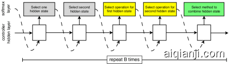
Each cell receives as input two initial hidden states h_i and h_(i−1) which are the outputs of two cells in previous two lower layers or the input image. The job of the controller RNN is to recursively predict the rest of the structure of the convolutional cell (Figure 3). The predictions of the controller for each cell are grouped into B blocks, where each block has 5 prediction steps made by 5 distinct softmax classifiers corresponding to discrete choices of the elements of a block:

在我们的搜索空间中，每个单元接收为输入两个初始隐藏状态$ h_i $和$ h_{i-1} $，它们是前两个较低层中两个单元的输出或输入图像的输出。考虑到这两个初始隐藏状态（FigureCell），控制器RNN递归地预测卷积单元的其余结构。每个单元的控制器的预测被分组为$ B $块，其中每个块具有5个预测步骤，该预测步骤由5个不同的Softmax分类器进行，这些分类器对应于块元素的离散选择：

该算法附加新创建的隐藏状态，将现有隐藏状态集作为后续块中的潜在输入。

1. Select a hidden state from h or from the set of hidden states created in previous blocks.
2. Select a second hidden state from the same options as in Step 1.
3. Select an operation to apply to the hidden state selected in Step 1.
4. Select an operation to apply to the hidden state selected in Step 2.
5. Select a method to combine the outputs of Step 3 and 4 to create a new hidden state.

1 从H或从之前创建的一组隐藏状态的块中获取中选择一个隐藏状态。

2 从与步骤1相同的选项中选择第二个隐藏状态。

3 选择一个操作以应用于在步骤1中选择的隐藏状态。

4 选择一个操作以应用于在步骤2中选择的隐藏状态。

5 选择一种方法来组合步骤3和4的输出以创建新的隐藏状态。

|

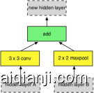
Figure 3: Controller model architecture for recursively constructing one block of a convolutional cell. Each block requires selecting 5 discrete parameters, each of which corresponds to the output of a softmax layer. Example constructed block shown on right. A convolutional cell contains B blocks, hence the controller contains 5B softmax layers for predicting the architecture of a convolutional cell. In our experiments, the number of blocks B is 5.1. [itemindent=0.7cm,label=Step 0.]

图3：用于递归构造卷积单元的一个块的控制器模型架构。每个模块需要选择5个离散参数，每个参数对应于softmax层的输出。右侧显示的示例构造块。卷积单元包含B 块，因此控制器包含
5B 用于预测卷积单元结构的softmax层。在我们的实验中，块数 B 是5

The algorithm appends the newly-created hidden state to the set of existing hidden states as a potential input in subsequent blocks. The controller RNN repeats the above 5 prediction steps B times corresponding to the B blocks in a convolutional cell. In our experiments, selecting B=5 provides good results, although we have not exhaustively searched this space due to computational limitations.

该算法将新创建的隐藏状态附加到现有隐藏状态的集合中，作为后续块中的潜在输入。控制器RNN对应一个卷积单元中的B个模块 重复上述5个预测步骤 B次。在我们的实验中，选择B=5 提供了良好的结果，尽管由于计算限制，我们尚未详尽搜索此空间。

在步骤3和4中，控制器RNN选择要应用于隐藏状态的操作。我们根据CNN文献中的患病率收集了以下一组操作：
In steps 3 and 4, the controller RNN selects an operation to apply to the hidden states. We collected the following set of operations based on their prevalence in the CNN literature:

∙ identity	∙ 1x3 then 3x1 convolution
∙ 1x7 then 7x1 convolution	∙ 3x3 dilated convolution
∙ 3x3 average pooling	∙ 3x3 max pooling
∙ 5x5 max pooling	∙ 7x7 max pooling
∙ 1x1 convolution	∙ 3x3 convolution
∙ 3x3 separable convolution	∙ 5x5 separable convolution
∙ 7x7 separable convolution

In our experiments, we apply each separable operation twice during the execution of the child model, once that operation is selected by the controller.

In step 5 the controller RNN selects a method to combine the two hidden states, either (1) elementwise addition between two hidden states and (2) concatenation between two hidden states along the filter dimension. Finally, all of the unused hidden states generated in the convolutional cell are concatenated together in depth to provide the final cell output.

To have the controller RNN predict both the Normal and Reduction cell we simply make the controller have 2×5B predictions in total, where the first 5B predictions are for the Normal Cell and the second 5B predictions are for the Reduction Cell.

在我们的实验中，一旦子模型被控制器选择，我们在子模型的执行过程中将每个可分离的操作应用两次。

在步骤5中，控制器RNN选择一种方法来组合两个隐藏状态，或者是（1）两个隐藏状态之间的逐元素相加，以及（2）沿着滤波器维度的两个隐藏状态之间的级联。最后，在卷积单元中生成的所有未使用的隐藏状态在深度上被串联在一起，以提供最终的单元输出。

为了让控制器RNN预测正态和归约单元，我们只需使控制器具有 2 ×5B个的预测，第一个 5B 预测是针对正常细胞单元，第二个 5B 预测是针对还原细胞单元的。

3 EXPERIMENTS AND RESULTS 实验与结果

In this section, we describe our experiments with Neural Architecture Search using the search space described above to learn a convolutional cell. In summary, all architecture searches are performed using the CIFAR-10 classification task (Krizhevsky, 2009). The controller RNN was trained using Proximal Policy Optimization (PPO) (Schulman et al., 2015) by employing a global workqueue system for generating a pool of child networks controlled by the RNN. In our experiments, the pool of workers in the workqueue consisted of 450 GPUs. Please see Appendix A for complete details of the architecture learning and controller system.

在本节中，我们将使用上述搜索空间来学习卷积单元，以神经结构搜索描述我们的实验。总之，所有架构搜索都是使用CIFAR-10分类任务执行的（Krizhevsky，2009年）。通过使用全局工作队列系统生成由RNN控制的子网络池，使用近端策略优化（PPO）对控制器RNN进行了培训（Schulman等，2015）。在我们的实验中，工作队列中的工人池由450个GPU组成。有关架构学习和控制器系统的完整详细信息，请参见附录A。

The result of this search process yields several candidate convolutional cells. Figure 4 shows a diagram of the top performing cell. Note the prevalence of separable convolutions and the number of branches as compared with competing architectures Simonyan and Zisserman (2014); Szegedy et al. (2015); He et al. (2016); Szegedy et al. (2016b, a). Subsequent experiments focus on this convolutional cell architecture, although we examine the efficacy of other, top-ranked convolutional cells in ImageNet experiments (described in Appendix B) and report their results as well. We call the three networks constructed from the best three cells NASNet-A, NASNet-B and NASNet-C.

该搜索过程的结果产生了几个候选卷积单元。图4显示了性能最高的单元图。注意与竞争性架构Simonyan和Zisserman（2014）相比，可分卷积的普遍性和分支的数量；塞格迪（Szegedy）等人。（2015）; 他等。（2016）; 塞格迪（Szegedy）等人。（2016b，a）。尽管我们检查了ImageNet实验中其他排名最高的卷积细胞的功效（在附录B中进行了描述），但随后的实验仍专注于这种卷积细胞体系结构，并报告了其结果。我们称由最好的三个单元构成的三个网络NASNet-A，NASNet-B和NASNet-C。

Figure 4: Architecture of the best convolutional cells (NASNet-A) with B=5 blocks identified with CIFAR-10 . The input (white) is the hidden state from previous activations (or input image). The output (pink) is the result of a concatenation operation across all resulting branches. Each convolutional cell is the result of B blocks. A single block is corresponds to two primitive operations (yellow) and a combination operation (green). Note that colors correspond to operations in Figure 3.

图4：最佳卷积单元（NASNet-A）的架构B=5用CIFAR-10标识的块。输入（白色）是先前激活（或输入图像）的隐藏状态。输出（粉红色）是跨所有结果分支进行串联操作的结果。每个卷积单元是乙块。单个块对应于两个基本操作（黄色）和组合操作（绿色）。注意，颜色与图3中的操作相对应。

We demonstrate the utility of the convolutional cell by employing this learned architecture on CIFAR-10 and a family of ImageNet classification tasks. The latter family of tasks is explored across a few orders of magnitude in computational budget. After having learned the convolutional cell, several hyper-parameters may be explored to build a final network for a given task: (1) the number of cell repeats N and (2) the number of filters in the initial convolutional cell. We employ a common heuristic to double the number of filters whenever the stride is 2.

我们通过在CIFAR-10和一系列ImageNet分类任务上采用这种学习的体系结构，展示了卷积单元的实用性。后一个任务系列的计算预算跨越了几个数量级。在学习了卷积单元之后，可以探索几个超参数来为给定任务构建最终的网络：（1）单元重复的次数ñ（2）初始卷积像元中的滤波器数量。每当步幅为2时，我们采用一种常见的启发式方法将过滤器数量加倍。

3.1GENERAL TRAINING STRATEGIES 通用训练策略

We found that adding Batch Normalization and/or a ReLU between the depthwise and pointwise operations in the separable convolution operations to not help performance. L1 regularization was tried with the NASNet models, but this was found to hurt performance. We also tried ELU Clevert et al. (2015) instead of ReLUs and found that performance was about the same. Dropout Srivastava et al. (2014) was also tried on the convolutional filters, but this was found to degrade performance.

我们发现在可分离的卷积运算中的深度运算和点运算之间添加批处理规范化和/或ReLU对性能没有帮助。使用NASNet模型尝试了L1正则化，但是发现这会损害性能。我们还尝试了ELU Clevert等。（2015）而不是ReLUs，发现性能大致相同。辍学 Srivastava等。（2014）还对卷积滤波器进行了尝试，但是发现这会降低性能。

Operation Ordering:

All convolution operations that could be predicted are applied within the convolutional cells in the following order: ReLU, convolution operation, Batch Normalization. We found this order to improve performance over a different ordering: convolution operation, Batch Normalization and ReLU. This result is inline with findings from other papers where using the pre-ReLU activation works better. In order to be sure shapes always match in the convolutional cells, 1x1 convolutions are inserted as necessary.

操作顺序：

可以预测的所有卷积运算都按以下顺序应用于卷积单元中：ReLU，卷积运算，批归一化。我们发现此顺序可以通过不同的顺序来提高性能：卷积运算，批处理规范化和ReLU。该结果与其他论文的研究结果一致，在这些论文中，使用Pre-ReLU激活效果更好。为了确保形状始终在卷积单元中匹配，根据需要插入1x1卷积。

Cell Path Dropout:

When training our NASNet models, we found stochastically dropping out each path (edge with a yellow box) in the cell with some fixed probability to be an extremely good regularizer. This is similar to Huang et al. (2016c) and Zhang et al. (2016) where they dropout full parts of their model during training and then at test time scale the path by the probability of keeping that path during training. Interestingly we found that linearly increasing the probability of dropping out a path over the course of training to significantly improve the final performance for both CIFAR and ImageNet experiments.

单元路径dropout：

在训练我们的NASNet模型时，我们发现以固定的概率随机丢弃单元中的每个路径（带有黄色框的边缘）是一个非常好的正则化器。这类似于Huang等。（2016c）和Zhang等。（2016），他们在训练过程中丢弃模型的全部部分，然后在测试时通过训练过程中保持该路径的概率来缩放路径。有趣的是，我们发现在训练过程中线性增加退出路径的可能性可以显着提高CIFAR和ImageNet实验的最终性能。

3.2RESULTS ON CIFAR-10 IMAGE CLASSIFICATION CIFAR-10图像分类的结果

For the task of image classification with CIFAR-10, we set N=4 or 6 (Figure 2). The networks are trained on CIFAR-10 for 600 epochs. The test accuracies of the best architectures are reported in Table 1 along with other state-of-the-art models; the best architectures found by the controller RNN are better than the previous state-of-the-art Shake-Shake model when comparing with the same number of parameters. Additionally, we only train for a third of the time where Shake-Shake trains for 1800 epochs. See appendix A for more details on CIFAR training.

对于使用CIFAR-10进行图像分类的任务，我们设置N = 4或6（图2）。在CIFAR-10上对网络进行了600个时期的培训。表1列出了最佳架构的测试准确性 以及其他最新模型。与相同数量的参数进行比较时，控制器RNN所找到的最佳架构要优于以前的最新Shake-Shake模型。此外，我们只训练“Shake-Shake”1800 epochs 的三分之一的时间。有关CIFAR训练的更多详细信息，请参见附录A。

Model	Depth	# parameters	Error rate (%)
DenseNet (L=40,k=12) (Huang et al., 2016a)	40	1.0M	5.24
DenseNet(L=100,k=12) (Huang et al., 2016a)	100	7.0M	4.10
DenseNet (L=100,k=24) (Huang et al., 2016a)	100	27.2M	3.74
DenseNet-BC (L=100,k=40) (Huang et al., 2016b)	190	25.6M	3.46
Shake-Shake 26 2x32d (Gastaldi, 2017)	26	2.9M	3.55
Shake-Shake 26 2x96d (Gastaldi, 2017)	26	26.2M	2.86
NAS v1 no stride or pooling (Zoph and Le, 2017)	15	4.2M	5.50
NAS v2 predicting strides (Zoph and Le, 2017)	20	2.5M	6.01
NAS v3 max pooling (Zoph and Le, 2017)	39	7.1M	4.47
NAS v3 max pooling + more filters (Zoph and Le, 2017)	39	37.4M	3.65
NASNet-A	N=6	3.3M	3.41
NASNet-B	N=4	2.6M	3.73
NASNet-C	N=4	3.1M	3.59

Table 1: Performance of Neural Architecture Search and other state-of-the-art models on CIFAR-10.
表1： CIFAR-10上神经体系结构搜索和其他最新模型的性能。

3.3 RESULTS ON IMAGENET IMAGE CLASSIFICATION IMAGENET图像分类的结果

We performed several sets of experiments on ImageNet with the best convolutional cells learned from CIFAR-10. Results are summarized in Table 2 and 3 and Figure 5. In the first set of experiments, we train several image classification systems operating on 299x299 or 331x331 resolution images scaled in computational demand on par with Inception-v2 Ioffe and Szegedy (2015), Inception-v3 Szegedy et al. (2016b) and PolyNet Zhang et al. (2016). We demonstrate that this family of models achieve state-of-the-art performance with fewer floating point operations and parameters than comparable architectures. Second, we demonstrate that by adjusting the scale of the model we can achieve state-of-the-art performance at smaller computational budgets, exceeding streamlined CNNs hand-designed for this operating regime Howard et al. (2017); Zhang et al. (2017).

Note we do not have residual connections around convolutional cells as the models learn skip connections on their own. We empirically found manually inserting residual connections between cells to not help performance. Our training setup on ImageNet is similar to Szegedy et al. (2016b), but please see Appendix A for details.

我们在ImageNet上进行了几组实验，使用了从CIFAR-10获得的最佳卷积单元。结果总结在表2和3以及图5中。在第一组实验中，我们训练了几个可在299x299或331x331分辨率图像上运行的图像分类系统，这些图像按计算需求按Inception-v2 Ioffe和Szegedy（2015），Inception-v3 Szegedy等人的水平进行缩放。（2016b）和PolyNet Zhang等人。（2016年）。我们证明，与同类架构相比，该系列模型以更少的浮点运算和参数实现了最先进的性能。其次，我们证明了通过调整模型的规模，我们可以在较小的计算预算下达到最新的性能，超过了为该操作方案手工设计的简化的CNN 。（2017）; 张等。（2017年）。

请注意，在卷积单元周围没有剩余连接，因为模型是自己学习跳跃连接的。根据经验，我们发现手动在单元之间插入剩余连接对性能没有帮助。我们在ImageNet上的培训设置类似于Szegedy等人。（2016b），但有关详细信息，请参见附录A。

|

Figure 5: Accuracy versus computational demand (left) and number of parameters (right) across top performing CNN architectures on ImageNet 2012 ILSVRC challenge prediction task (compiled as of July 2017). Computational demand is measured in the number of floating-point multiply-add operations to process a single image. Black circles indicate previously published work and red squares highlight our proposed models. Vertical dashed line indicates 1 billion multiply-add operations. Horizontal dashed line indicates 80% precision@1 prediction accuracy.

Model	image size	# parameters	Mult-Adds	Top 1 Acc. (%)	Top 5 Acc. (%)
Inception V2 (Ioffe and Szegedy, 2015)	224×224	11.2 M	1.94 B	74.8	92.2
NASNet-A (N = 5)	299×299	10.9 M	2.35 B	78.6	94.2
Inception V3 (Szegedy et al., 2016b)	299×299	23.8 M	5.72 B	78.0	93.9
Xception (Chollet, 2016)	299×299	22.8 M	8.38 B	79.0	94.5
Inception ResNet V2 (Szegedy et al., 2016a)	299×299	55.8 M	13.2 B	80.4	95.3
NASNet-A (N = 7)	299×299	22.6 M	4.93 B	80.8	95.3
ResNeXt-101 (64 x 4d) (Xie et al., 2016)	320×320	83.6 M	31.5 B	80.9	95.6
PolyNet (Zhang et al., 2016)	331×331	92 M	34.7 B	81.3	95.8
DPN-131 (Chen et al., 2017)	320×320	79.5 M	32.0 B	81.5	95.8
NASNet-A (N = 7)	331×331	84.9 M	23.2 B	82.3	96.0

Table 2: Performance of architecture search and other state-of-the-art models on ImageNet classification. Mult-Adds indicate the number of composite multiply-accumulate operations for a single image.

表2：关于ImageNet分类的体系结构搜索和其他最新模型的性能。Mult-Adds表示单个图像的合成乘法累加运算的数量。

Model	# parameters	Mult-Adds	Top 1 Acc. (%)	Top 5 Acc. (%)
Inception V1 (Szegedy et al., 2015)	6.6M	1,448 M	69.8	89.9
MobileNet-224 Howard et al. (2017)	4.2 M	569 M	70.6	89.5
ShuffleNet (2x) Zhang et al. (2017)	∼ 5M	524 M	70.9	89.8
NASNet-A (N=4)	5.3 M	564 M	74.0	91.6
NASNet-B (N=4)	5.3M	488 M	72.8	91.3
NASNet-C (N=3)	4.9M	558 M	72.5	91.0

Table 3: Performance on ImageNet classification on a subset of models operating in a constrained computational setting, i.e., <1.5 B multiply-accumulate operations per image. All models employ 224x224 images.

表3：在受约束的计算设置下运行的模型子集上ImageNet分类的性能，即<1.5 B每个图像的乘法累加运算。所有型号均使用224x224图像。

Table 2 shows that the convolutional cells discovered with CIFAR-10 generalize well to ImageNet problems. In particular, each model based on the convolutional cell exceeds the predictive performance of the corresponding hand-designed model. Importantly, the largest model achieves a new state-of-the-art performance for ImageNet (82.3%) based on single, non-ensembled predictions, surpassing previous state-of-the-art by 0.8% Chen et al. (2017). Figure 5 shows a complete summary of these results. Note the family of models based on convolutional cells provides an envelope over a broad class of human-invented architectures.

表 2显示，用CIFAR-10发现的卷积单元可以很好地推广到ImageNet问题。特别是，基于卷积单元的每个模型都超过了相应的手工设计模型的预测性能。重要的是，最大的模型基于单个非组合的预测，实现了ImageNet的最新技术性能（82.3％），比之前的最新技术提高了0.8％（Chen等人）。（2017年）。图5显示了这些结果的完整摘要。请注意，基于卷积单元的模型家族为人类发明的各种体系结构提供了一个包络。

Finally, we test how well the best convolutional cells may perform in a resource-constrained setting, e.g., mobile devices (Table 3). In these settings, the number of floating point operations is severely constrained and predictive performance must be weighed against latency requirements on a device with limited computational resources. MobileNet Howard et al. (2017) and ShuffleNet Zhang et al. (2017) provide state-of-the-art results predicting 70.6% and 70.9% accuracy, respectively on 224x224 images using ∼ 550M multliply-add operations. An architecture constructed from the best convolutional cells achieves superior predictive performance (74.0% accuracy) surpassing previous models but with comparable computational demand. In summary, we find that the learned convolutional cells are flexible across model scales achieving state-of-the-art performance across almost 2 orders of magnitude in computational budget.

最后，我们测试最佳卷积单元在资源受限的环境（例如移动设备）中的性能如何（表3）。在这些设置中，浮点运算的数量受到严格限制，并且必须在计算资源有限的设备上，将预测性能与延迟要求进行权衡。MobileNet Howard等。（2017）和ShuffleNet Zhang等人。（2017）提供了预测70.6％和70.9的最新结果
％ 分别使用224x224图像的精度 〜550M多加运算。由最佳卷积单元构建的体系结构可实现超越先前模型的出色预测性能（准确度为74.0％），但具有可比的计算需求。总而言之，我们发现学习的卷积单元在模型规模上很灵活，在计算预算中几乎达到了两个数量级，从而实现了最新的性能。

4 RELATED WORK

The proposed method is related to previous work in hyperparameter optimization (Pinto et al., 2009; Bergstra et al., 2011; Bergstra and Bengio, 2012; Snoek et al., 2012, 2015; Bergstra et al., 2013; Mendoza et al., 2016) – especially recent approaches in designing architectures such as Neural Fabrics (Saxena and Verbeek, 2016), DiffRNN (Miconi, 2016), MetaQNN (Baker et al., 2016) and DeepArchitect (Negrinho and Gordon, 2017). A more flexible class of methods for designing architecture is evolutionary algorithms (Wierstra et al., 2005; Floreano et al., 2008; Stanley et al., 2009; Jozefowicz et al., 2015; Real et al., 2017; Miikkulainen et al., 2017; Xie and Yuille, 2017), yet they have not had as much success at large scale. Xie and Yuille (2017) also transferred learned architectures from CIFAR-10 to ImageNet but performance of these models (top-1 accuracy 72.1%) are notably below previous state-of-the-art (Table 2).

The concept of having one neural network interact with a second neural network to aid the learning process, or learning to learn or meta-learning (Hochreiter et al., 2001; Schaul and Schmidhuber, 2010) has attracted much attention in recent years (Andrychowicz et al., 2016; Wang et al., 2016; Duan et al., 2016; Ha et al., 2017; Li and Malik, 2017; Ravi and Larochelle, 2017; Finn et al., 2017). Most of these approaches have not been scaled to large problems like ImageNet. A notable exception is recent work focused on learning an optimizer for ImageNet classification that achieved notable improvements (Wichrowska et al., 2017).

The design of our search space took much inspiration from LSTMs (Hochreiter and Schmidhuber, 1997), and NASCell (Zoph and Le, 2017). The modular structure of the convolutional cell is also related to previous methods on ImageNet such as VGG (Simonyan and Zisserman, 2014), Inception (Szegedy et al., 2015, 2016b, 2016a), ResNet/ResNext (He et al., 2016; Xie et al., 2016), and Xception/MobileNet (Chollet, 2016; Howard et al., 2017).

所提出的方法与以前的工作在超参数优化 （平托等人，2009年; Bergstra等人，2011 ; Bergstra和Bengio，2012 ;斯诺克等人，2012，2015年; Bergstra等人，2013 ; Mendoza等等人，2016年） –特别是设计架构的最新方法，例如神经织物 （Saxena和Verbeek，2016年），DiffRNN （Miconi，2016年），MetaQNN （Baker等人，2016年）和DeepArchitect （ Negrinho 和Gordon，2017年）。用于设计架构的一类更灵活的方法是进化算法（Wierstra等人，2005 ; Floreano等人，2008 ; Stanley等人，2009 ; Jozefowicz等人，2015 ; Real等人，2017 ; Miikkulainen等人等人，2017年； Xie和Yuille，2017年），但他们在大规模方面还没有取得太大的成功。 Xie和Yuille（2017）也将学习的架构从CIFAR-10转移到了ImageNet，但是这些模型的性能（最高1位准确性为72.1％）明显低于以前的最新技术水平（表2）。

具有一个神经网络与另一个神经网络交互以辅助学习过程，学习或元学习的概念（Hochreiter等人，2001； Schaul和Schmidhuber，2010）近年来引起了很多关注 （Andrychowicz等人，2016 ; Wang等，2016 ; Duan等，2016 ; Ha等，2017 ; Li和Malik，2017 ; Ravi和Larochelle，2017 ; Finn等，2017）。这些方法大多数都没有扩展到像ImageNet这样的大问题。一个明显的例外是最近的工作专注于学习ImageNet分类的优化器，该优化器取得了显着的改善（Wichrowska等人，2017）。

我们的搜索空间设计从LSTM （Hochreiter和Schmidhuber，1997）和NASCell （Zoph和Le，2017）中获得了很多启发 。卷积单元的模块化结构也与上ImageNet以前的方法，如VGG （西蒙尼扬和Zisserman，2014），启 （Szegedy等人，2015，2016B，2016a），RESNET / ResNext （He等人，2016； Xie等人，2016年）和Xception / MobileNet （Chollet，2016年； Howard等人，2017年）。

5 CONCLUSION

In this work, we demonstrate how to learn scalable, convolutional cells from data that transfer to multiple image classification tasks. The key insight to this approach is to design a search space that decouples the complexity of an architecture from the depth of a network. This resulting search space permits identifying good architectures on a small dataset (i.e., CIFAR-10) and transferring the learned architecture to image classifications across a range of data and computational scales.

The resulting architectures approach or exceed state-of-the-art performance in terms of CIFAR-10, ImageNet classification with less computational demand than human-designed architectures Szegedy et al. (2016b); Ioffe and Szegedy (2015); Zhang et al. (2016). The ImageNet results are particularly important because many state-of-the-art computer vision problems (e.g., object detection Huang et al. (2016d), face detection Schroff et al. (2015), image localization Weyand et al. (2016)) derive image features or architectures from ImageNet classification models. Finally, we demonstrate that we can employ the resulting learned architecture to perform ImageNet classification with reduced computational budgets that outperform streamlined architectures targeted to mobile and embedded platforms Howard et al. (2017); Zhang et al. (2017).

Our results have strong implications for transfer learning and meta-learning as this is the first work to demonstrate state-of-the-art results using meta-learning on a large scale problem. This work also highlights that learned elements of network architectures, beyond model weights, can transfer across datasets.

在这项工作中，我们演示了如何从传输到多个图像分类任务的数据中学习可伸缩的卷积单元。这种方法的关键见解是设计一个搜索空间，该空间将体系结构的复杂性与网络的深度脱钩。该结果搜索空间允许在小型数据集（即CIFAR-10）上标识良好的体系结构，并将学习到的体系结构迁移到更大的数据和计算范围的图像分类。

与人工设计的体系结构相比，生成的体系结构在CIFAR-10，ImageNet分类方面的性能达到或超过了最新技术水平，而计算需求却低于人工设计的体系结构。（2016b）; 艾菲和塞格迪（2015）; 张等。（2016）。ImageNet的结果特别重要，因为存在许多最新的计算机视觉问题（例如，物体检测Huang等人（2016d），人脸检测Schroff等人（2015），图像定位Weyand等人（2016））从ImageNet分类模型中得出图像特征或体系结构。最后，我们证明了我们可以使用所得的学习型架构以减少的计算预算来执行ImageNet分类，其性能优于针对移动平台和嵌入式平台的精简架构Howard等人。（2017）; 张等。（2017年）。

我们的研究结果对迁移学习和元学习具有重要的意义，因为这是首次证明在大规模问题上使用元学习展示最新结果的工作。这项工作还强调，除了模型权重之外，网络体系结构的学习元素还可以跨数据集进行迁移。

ACKNOWLEDGEMENTS
We thank Jeff Dean, Yifeng Lu, Jonathan Shen, Vishy Tirumalashetty, Xiaoqiang Zheng, and the Google Brain team for the help with the project. We additionally thank Christian Sigg for performance improvements to depthwise separable convolutions.

致谢
我们感谢Jeff Dean，Lu Yifeng Lu，Jonathan Shen，Vishy Tirumalashetty，Zhengqiang Zheng和Google Brain团队为该项目提供的帮助。我们还要感谢Christian Sigg对深度可分离卷积的性能改进。
REFERENCES
Andrychowicz et al. (2016) Marcin Andrychowicz, Misha Denil, Sergio Gomez, Matthew W. Hoffman, David Pfau, Tom Schaul, and Nando de Freitas. Learning to learn by gradient descent by gradient descent. In Advances in Neural Information Processing Systems, pages 3981–3989, 2016.
Ba et al. (2016) Jimmy Lei Ba, Jamie Ryan Kiros, and Geoffrey E Hinton. Layer normalization. arXiv preprint arXiv:1607.06450, 2016.
Baker et al. (2016) Bowen Baker, Otkrist Gupta, Nikhil Naik, and Ramesh Raskar. Designing neural network architectures using reinforcement learning. In International Conference on Learning Representations, 2016.
Bergstra and Bengio (2012) James Bergstra and Yoshua Bengio. Random search for hyper-parameter optimization. Journal of Machine Learning Research, 2012.
Bergstra et al. (2011) James Bergstra, Rémi Bardenet, Yoshua Bengio, and Balázs Kégl. Algorithms for hyper-parameter optimization. In Neural Information Processing Systems, 2011.
Bergstra et al. (2013) James Bergstra, Daniel Yamins, and David D. Cox. Making a science of model search: Hyperparameter optimization in hundreds of dimensions for vision architectures. International Conference on Machine Learning, 2013.
Chen et al. (2016) Jianmin Chen, Rajat Monga, Samy Bengio, and Rafal Jozefowicz. Revisiting distributed synchronous sgd. In International Conference on Learning Representations Workshop Track, 2016.
Chen et al. (2017) Yunpeng Chen, Jianan Li, Huaxin Xiao, Xiaojie Jin, Shuicheng Yan, and Jiashi Feng. Dual path networks. arXiv preprint arXiv:1707.01083, 2017.
Chollet (2016) François Chollet. Xception: Deep learning with depthwise separable convolutions. arXiv preprint arXiv:1610.02357, 2016.
Clevert et al. (2015) Djork-Arné Clevert, Thomas Unterthiner, and Sepp Hochreiter. Fast and accurate deep network learning by exponential linear units (elus). arXiv preprint arXiv:1511.07289, 2015.
Deng et al. (2009) Jia Deng, Wei Dong, Richard Socher, Li-Jia Li, Kai Li, and Li Fei-Fei. Imagenet: A large-scale hierarchical image database. In IEEE Conference on Computer Vision and Pattern Recognition. IEEE, 2009.
Donahue et al. (2014) Jeff Donahue, Yangqing Jia, Oriol Vinyals, Judy Hoffman, Ning Zhang, Eric Tzeng, and Trevor Darrell. Decaf: A deep convolutional activation feature for generic visual recognition. In Icml, volume 32, pages 647–655, 2014.
Duan et al. (2016) Yan Duan, John Schulman, Xi Chen, Peter L Bartlett, Ilya Sutskever, and Pieter Abbeel. RL
2
: Fast reinforcement learning via slow reinforcement learning. arXiv preprint arXiv:1611.02779, 2016.
Finn et al. (2017) Chelsea Finn, Pieter Abbeel, and Sergey Levine. Model-agnostic meta-learning for fast adaptation of deep networks. arXiv preprint arXiv:1703.03400, 2017.
Floreano et al. (2008) Dario Floreano, Peter Dürr, and Claudio Mattiussi. Neuroevolution: from architectures to learning. Evolutionary Intelligence, 2008.
Fukushima (1980) Kunihiko Fukushima. A self-organizing neural network model for a mechanism of pattern recognition unaffected by shift in position. Biological Cybernetics, page 93–202, 1980.
Gastaldi (2017) Xavier Gastaldi. Shake-shake regularization of 3-branch residual networks. In International Conference on Learning Representations Workshop Track, 2017.
Ha et al. (2017) David Ha, Andrew Dai, and Quoc V. Le. Hypernetworks. In International Conference on Learning Representations, 2017.
He et al. (2016) Kaiming He, Xiangyu Zhang, Shaoqing Ren, and Jian Sun. Deep residual learning for image recognition. In IEEE Conference on Computer Vision and Pattern Recognition, 2016.
Hochreiter and Schmidhuber (1997) Sepp Hochreiter and Juergen Schmidhuber. Long short-term memory. Neural Computation, 1997.
Hochreiter et al. (2001) Sepp Hochreiter, A Younger, and Peter Conwell. Learning to learn using gradient descent. Artificial Neural Networks, pages 87–94, 2001.
Howard et al. (2017) Andrew G Howard, Menglong Zhu, Bo Chen, Dmitry Kalenichenko, Weijun Wang, Tobias Weyand, Marco Andreetto, and Hartwig Adam. Mobilenets: Efficient convolutional neural networks for mobile vision applications. arXiv preprint arXiv:1704.04861, 2017.
Huang et al. (2016a) Gao Huang, Zhuang Liu, and Kilian Q. Weinberger. Densely connected convolutional networks. arXiv preprint arXiv:1608.06993, 2016a.
Huang et al. (2016b) Gao Huang, Zhuang Liu, Kilian Q. Weinberger, and Laurens van der Maaten. Densely connected convolutional networks. arXiv preprint arXiv:1608.06993, 2016b.
Huang et al. (2016c) Gao Huang, Yu Sun, Zhuang Liu, Daniel Sedra, and Kilian Weinberger. Deep networks with stochastic depth. arXiv preprint arXiv:1603.09382, 2016c.
Huang et al. (2016d) Jonathan Huang, Vivek Rathod, Chen Sun, Menglong Zhu, Anoop Korattikara, Alireza Fathi, Ian Fischer, Zbigniew Wojna, Yang Song, Sergio Guadarrama, et al. Speed/accuracy trade-offs for modern convolutional object detectors. arXiv preprint arXiv:1611.10012, 2016d.
Ioffe and Szegedy (2015) Sergey Ioffe and Christian Szegedy. Batch normalization: Accelerating deep network training by reducing internal covariate shift. In ICML, 2015.
Jozefowicz et al. (2015) Rafal Jozefowicz, Wojciech Zaremba, and Ilya Sutskever. An empirical exploration of recurrent network architectures. In ICML, 2015.
Krizhevsky (2009) Alex Krizhevsky. Learning multiple layers of features from tiny images. Technical report, University of Toronto, 2009.
Krizhevsky et al. (2012) Alex Krizhevsky, Ilya Sutskever, and Geoffrey E. Hinton. Imagenet classification with deep convolutional neural networks. In Advances in Neural Information Processing System, 2012.
LeCun et al. (1998) Yann LeCun, Léon Bottou, Yoshua Bengio, and Patrick Haffner. Gradient-based learning applied to document recognition. Proceedings of the IEEE, 1998.
Li and Malik (2017) Ke Li and Jitendra Malik. Learning to optimize neural nets. arXiv preprint arXiv:1703.00441, 2017.
Mendoza et al. (2016) Hector Mendoza, Aaron Klein, Matthias Feurer, Jost Tobias Springenberg, and Frank Hutter. Towards automatically-tuned neural networks. In Proceedings of the 2016 Workshop on Automatic Machine Learning, pages 58–65, 2016.
Miconi (2016) Thomas Miconi. Neural networks with differentiable structure. arXiv preprint arXiv:1606.06216, 2016.
Miikkulainen et al. (2017) Risto Miikkulainen, Jason Liang, Elliot Meyerson, Aditya Rawal, Dan Fink, Olivier Francon, Bala Raju, Arshak Navruzyan, Nigel Duffy, and Babak Hodjat. Evolving deep neural networks. arXiv preprint arXiv:1703.00548, 2017.
Negrinho and Gordon (2017) Renato Negrinho and Geoff Gordon. DeepArchitect: Automatically designing and training deep architectures. arXiv preprint arXiv:1704.08792, 2017.
Pinto et al. (2009) Nicolas Pinto, David Doukhan, James J DiCarlo, and David D Cox. A high-throughput screening approach to discovering good forms of biologically inspired visual representation. PLoS Computational Biology, 5(11):e1000579, 2009.
Ravi and Larochelle (2017) Sachin Ravi and Hugo Larochelle. Optimization as a model for few-shot learning. In International Conference on Learning Representations, 2017.
Real et al. (2017) Esteban Real, Sherry Moore, Andrew Selle, Saurabh Saxena, Yutaka Leon Suematsu, Quoc Le, and Alex Kurakin. Large-scale evolution of image classifiers. arXiv preprint arXiv:1703.01041, 2017.
Saxena and Verbeek (2016) Shreyas Saxena and Jakob Verbeek. Convolutional neural fabrics. In Advances in Neural Information Processing Systems, 2016.
Schaul and Schmidhuber (2010) Tom Schaul and Juergen Schmidhuber. Metalearning. Scholarpedia, 2010.
Schroff et al. (2015) Florian Schroff, Dmitry Kalenichenko, and James Philbin. Facenet: A unified embedding for face recognition and clustering. In Proceedings of the IEEE Conference on Computer Vision and Pattern Recognition, pages 815–823, 2015.
Schulman et al. (2015) John Schulman, Sergey Levine, Pieter Abbeel, Michael Jordan, and Philipp Moritz. Trust region policy optimization. In International Conference on Machine Learning, 2015.
Simonyan and Zisserman (2014) Karen Simonyan and Andrew Zisserman. Very deep convolutional networks for large-scale image recognition. arXiv preprint arXiv:1409.1556, 2014.
Snoek et al. (2012) Jasper Snoek, Hugo Larochelle, and Ryan P. Adams. Practical Bayesian optimization of machine learning algorithms. In Neural Information Processing Systems, 2012.
Snoek et al. (2015) Jasper Snoek, Oren Rippel, Kevin Swersky, Ryan Kiros, Nadathur Satish, Narayanan Sundaram, Mostofa Patwary, Mostofa Ali, Ryan P. Adams, et al. Scalable Bayesian optimization using deep neural networks. In International Conference on Machine Learning, 2015.
Srivastava et al. (2014) Nitish Srivastava, Geoffrey E Hinton, Alex Krizhevsky, Ilya Sutskever, and Ruslan Salakhutdinov. Dropout: a simple way to prevent neural networks from overfitting. Journal of Machine Learning Research, 15(1):1929–1958, 2014.
Stanley et al. (2009) Kenneth O. Stanley, David B. D’Ambrosio, and Jason Gauci. A hypercube-based encoding for evolving large-scale neural networks. Artificial Life, 2009.
Szegedy et al. (2015) Christian Szegedy, Wei Liu, Yangqing Jia, Pierre Sermanet, Scott Reed, Dragomir Anguelov, Dumitru Erhan, Vincent Vanhoucke, and Andrew Rabinovich. Going deeper with convolutions. In IEEE Conference on Computer Vision and Pattern Recognition, 2015.
Szegedy et al. (2016a) Christian Szegedy, Sergey Ioffe, Vincent Vanhoucke, and Alex Alemi. Inception-v4, inception-resnet and the impact of residual connections on learning. arXiv preprint arXiv:1602.07261, 2016a.
Szegedy et al. (2016b) Christian Szegedy, Vincent Vanhoucke, Sergey Ioffe, Jon Shlens, and Zbigniew Wojna. Rethinking the inception architecture for computer vision. In IEEE Conference on Computer Vision and Pattern Recognition, 2016b.
Wang et al. (2016) Jane X Wang, Zeb Kurth-Nelson, Dhruva Tirumala, Hubert Soyer, Joel Z Leibo, Remi Munos, Charles Blundell, Dharshan Kumaran, and Matt Botvinick. Learning to reinforcement learn. arXiv preprint arXiv:1611.05763, 2016.
Weyand et al. (2016) Tobias Weyand, Ilya Kostrikov, and James Philbin. Planet-photo geolocation with convolutional neural networks. arXiv preprint arXiv:1602.05314, 2016.
Wichrowska et al. (2017) Olga Wichrowska, Niru Maheswaranathan, Matthew W. Hoffman, Sergio Gomez Colmenarejo, Misha Denil, Nando de Freitas, and Jascha Sohl-Dickstein. Learned optimizers that scale and generalize. arXiv preprint arXiv:1703.04813, 2017.
Wierstra et al. (2005) Daan Wierstra, Faustino J. Gomez, and Jürgen Schmidhuber. Modeling systems with internal state using evolino. In The Genetic and Evolutionary Computation Conference, 2005.
Williams (1992) Ronald J. Williams. Simple statistical gradient-following algorithms for connectionist reinforcement learning. In Machine Learning, 1992.
Xie and Yuille (2017) Lingxi Xie and Alan Yuille. Genetic CNN. arXiv preprint arXiv:1703.01513, 2017.
Xie et al. (2016) Saining Xie, Ross Girshick, Piotr Dollár, Zhuowen Tu, and Kaiming He. Aggregated residual transformations for deep neural networks. arXiv preprint arXiv:1611.05431, 2016.
Zhang et al. (2017) Xiangyu Zhang, Xinyu Zhou, Lin Mengxiao, and Jian Sun. Shufflenet: An extremely efficient convolutional neural network for mobile devices. arXiv preprint arXiv:1707.01083, 2017.
Zhang et al. (2016) Xingcheng Zhang, Zhizhong Li, Chen Change Loy, and Dahua Lin. Polynet: A pursuit of structural diversity in very deep networks. arXiv preprint arXiv:1611.05725, 2016.
Zoph and Le (2017) Barret Zoph and Quoc V. Le. Neural architecture search with reinforcement learning. In International Conference on Learning Representations, 2017.

APPENDIX

APPENDIX A EXPERIMENTAL DETAILS

A.1DATASET FOR ARCHITECTURE SEARCH 数据集

The CIFAR-10 dataset [Krizhevsky, 2009] consists of 60,000 32x32 RGB images across 10 classes (50,000 train and 10,000 test images). We partition a random subset of 5,000 images from the training set to use as a validation set for the controller RNN. All images are whitened and then undergone several data augmentation steps: we randomly crop 32x32 patches from upsampled images of size 40x40 and apply random horizontal flips. This data augmentation procedure is common among related work.

CIFAR-10数据集 [Krizhevsky，2009 ]由10个类别的60,000个32x32 RGB图像组成（50,000个训练和10,000个测试图像）。我们从训练集中划分了5,000个图像的随机子集，以用作控制器RNN的验证集。所有图像均变白，然后经历几个数据增强步骤：我们从大小为40x40的上采样图像中随机裁剪32x32色块，并应用随机的水平翻转。这种数据扩充过程在相关工作中很常见。

A.2CONTROLLER ARCHITECTURE 控制器架构

The controller RNN is a one-layer LSTM [Hochreiter and Schmidhuber, 1997] with 100 hidden units at each layer and 2×5B softmax predictions for the two convolutional cells (where B is typically 5) associated with each architecture decision. Each of the 10B predictions of the controller RNN is associated with a probability. The joint probability of a child network is the product of all probabilities at these 10B softmaxes. This joint probability is used to compute the gradient for the controller RNN. The gradient is scaled by the validation accuracy of the child network to update the controller RNN such that the controller assigns low probabilities for bad child networks and high probabilities for good child networks.

Unlike Zoph and Le [2017], who used the REINFORCE rule [Williams, 1992] to update the controller, we employ Proximal Policy Optimization (PPO) [Schulman et al., 2015] with learning rate 0.00035 because it made training more robust and increased convergence speed. To encourage exploration we also use an entropy penalty with a weight of 0.00001. We also use a baseline function, which we set to be an exponential moving average of previous rewards, with a weight of 0.95. The weights of the controller are initialized uniformly between -0.1 and 0.1.

控制器RNN是一层LSTM [Hochreiter and Schmidhuber，1997 ]，每层有100个隐藏单元，2×5B 两个卷积像元的softmax预测（其中 B通常是5）与每个架构决策相关联。每一个10B控制器RNN的预测与概率相关。子网络的联合概率是这些条件下所有概率的乘积10乙softmaxes。该联合概率用于计算控制器RNN的梯度。通过子网络的验证精度对梯度进行缩放，以更新控制器RNN，以便控制器为不良子网络分配低概率，为不良子网络分配高概率。

与 Zoph和Le [ 2017 ]使用REINFORCE规则 [Williams，1992 ]更新控制器不同，我们采用学习率0.00035的近距离策略优化（PPO） [Schulman et al。，2015 ]，因为它使训练更加稳健，并且加快收敛速度​​。为了鼓励探索，我们还使用权重为0.00001的熵罚。我们还使用基线函数，将其设置为先前奖励的指数移动平均值，权重为0.95。控制器的权重在-0.1到0.1之间统一初始化。

A.3TRAINING OF THE CONTROLLER

For distributed training, we use a work queue system where all the samples generated from the controller RNN are added to a global workqueue. A free "child" worker in a distributed worker pool asks the controller for new work from the global workqueue. Once the training of the child network is complete, the accuracy on a held-out validation set is computed and reported to the controller RNN. In our experiments we use a child worker pool size of 450, which means there are 450 networks being trained on 450 GPUs concurrently at any time. Upon receiving enough child model training results, the Controller RNN will perform a gradient update on its weights using TRPO and then sample another batch of architectures that go into the global work queue. This process continues until a predetermined number of architectures have been sampled. In our experiments, this predetermined number of architectures is 20,000 which means the search process is terminated after 20,000 child models have been trained. Additionally, we update the controller RNN with minibatches of 20 architectures. Once the search is over, the top 250 architectures are then chosen to train until convergence on CIFAR-10 to determine the very best architecture.

对于分布式培训，我们使用工作队列系统，其中将从控制器RNN生成的所有样本都添加到全局工作队列中。分布式工作人员池中有一个免费的“儿童”工作人员，要求控制器从全局工作队列中请求新工作。子网络的训练完成后，将计算保留验证集的准确性，并将其报告给控制器RNN。在我们的实验中，我们使用了450个童工池，这意味着可以随时在450个GPU上同时训练450个网络。收到足够的子模型训练结果后，Controller RNN将使用TRPO对权重执行梯度更新，然后对进入全局工作队列的另一批体系结构进行采样。该过程一直持续到已经采样了预定数量的体系结构为止。在我们的实验中，该预定数量的体系结构为20,000，这意味着在训练了20,000个子模型之后，搜索过程将终止。此外，我们使用20种架构的微型批次更新了控制器RNN。搜索结束后，然后选择排名前250位的体系结构进行训练，直到在CIFAR-10上收敛，从而确定最佳体系结构。

A.4TRAINING OF CIFAR MODELS

All of our CIFAR models use a single period cosine decay as in Gastaldi [2017]. All models use the momentum optimizer with momentum rate set to 0.9. All models also use L2 weight decay. Each architecture is trained for a fixed 20 epochs on CIFAR-10 during the architecture search process. Additionally, we found it beneficial to use the cosine learning rate decay during the 20 epochs the CIFAR models were trained for as this helped to further differentiate good architectures. We also found that having the CIFAR models use a small N=2 during the architecture search process allowed for models to train quite quickly, while still finding cells that work well once more were stacked.
我们的所有CIFAR模型都使用单周期余弦衰减，如Gastaldi [ 2017 ]中所述。所有模型都使用动量优化器，并将动量率设置为0.9。所有型号还使用L2重量衰减。在架构搜索过程中，每种架构都在CIFAR-10上进行了固定的20个时期训练。此外，我们发现在训练CIFAR模型的20个时期内使用余弦学习速率衰减是有益的，因为这有助于进一步区分良好的体系结构。我们还发现，在架构搜索过程中，让CIFAR模型使用较小的N = 2可以使模型快速训练，同时仍然可以找到堆叠良好的单元。

A.5TRAINING OF IMAGENET MODELS

We use ImageNet 2012 ILSVRC challenge data for large scale image classification. The dataset consists of ∼ 1.2M images labeled across 1000 classes Deng et al. [2009]. Overall our training and testing procedures are almost identical to Szegedy et al. [2016b]. ImageNet models are trained and evaluated on 299x299 or 331x331 images using the same data augmentation procedures as described previously Szegedy et al. [2016b]. We use distributed synchronous SGD to train the ImageNet model with 50 workers (and 3 backup workers) each with a Tesla K40 GPU Chen et al. [2016]. We use RMSProp with a decay of 0.9 and epsilon of 1.0. Evaluations are calculated using with a running average of parameters over time with a decay rate of 0.9999. We use label smoothing with a value of 0.1 for all ImageNet models as done in Szegedy et al. [2016b]. Additionally, all models use an auxiliary classifier located at 2/3 of the way up the network. The loss of the auxiliary classifier is weighted by 0.4 as done in Szegedy et al. [2016b]. We empirically found our network to be insensitive to the number of parameters associated with this auxiliary classifier along with the weight associated with the loss. All models also use L2 regularization. The learning rate decay scheme is the exponential decay scheme used in Szegedy et al. [2016b]. Dropout is applied to the final softmax matrix with probability 0.5.
我们使用ImageNet 2012 ILSVRC挑战数据进行大规模图像分类。数据集包括〜跨1000个类别标记的120万张图片Deng等。[ 2009 ]。总体而言，我们的培训和测试程序几乎与Szegedy等人相同。[ 2016b ]。使用与之前Szegedy等人所述相同的数据增强程序，对299x299或331x331图像上的ImageNet模型进行训练和评估。[ 2016b ]。我们使用分布式同步SGD训练50名工人（和3名备用工人）的ImageNet模型，每个工人都配有Tesla K40 GPU Chen等。[ 2016年]。我们使用衰减为0.9且epsilon为1.0的RMSProp。使用随时间推移的参数的运行平均值（衰减率为0.9999）来计算评估。正如Szegedy等人所做的那样，我们对所有ImageNet模型使用的标签平滑值为0.1 。[ 2016b ]。此外，所有型号均使用位于网络上2/3处的辅助分类器。辅助分类器的损失按Szegedy等人的方法加权为0.4 。[ 2016b ]。我们凭经验发现我们的网络对与该辅助分类器关联的参数数量以及与损失关联的权重不敏感。所有模型还使用L2正则化。学习速率衰减方案是用于塞格迪（Szegedy）等人。[ 2016b ]。辍学率以0.5的概率应用于最终的softmax矩阵。

APPENDIX B ADDITIONAL EXPERIMENTS

We now present two additional cells that performed well on CIFAR and ImageNet. The search spaces used for these cells are slightly different than what was used for NASNet-A. For the NASNet-B model in Figure 6 we do not concatenate all of the unused hidden states generated in the convolutional cell. Instead all of the hiddenstates created within the convolutional cell, even if they are currently used, are fed into the next layer. Note that B=4 and there are 4 hiddenstates as input to the cell as these numbers must match for this cell to be valid. We also allow addition followed by layer normalization Ba et al. [2016] or instance normalization to be predicted as two of the combination operations within the cell, along with addition or concatenation.

Figure 6: Architecture of NASNet-B convolutional cell with B=4 blocks identified with CIFAR-10. The input (white) is the hidden state from previous activations (or input image). Each convolutional cell is the result of B blocks. A single block is corresponds to two primitive operations (yellow) and a combination operation (green). As do we not concatenate the output hidden states, each output hidden state is used as a hidden state in the future layers. Each cell takes in 4 hidden states and thus needs to also create 4 output hidden states. Each output hidden state is therefore labeled with 0, 1, 2, 3 to represent the next four layers in that order.Figure 7: Architecture of NASNet-C convolutional cell with B=4 blocks identified with CIFAR-10. The input (white) is the hidden state from previous activations (or input image). The output (pink) is the result of a concatenation operation across all resulting branches. Each convolutional cell is the result of B blocks. A single block corresponds to two primitive operations (yellow) and a combination operation (green).For NASNet-C (Figure 7), we concatenate all of the unused hidden states generated in the convolutional cell like in NASNet-A, but now we allow the prediction of addition followed by layer normalization or instance normalization like in NASNet-B.

其他实验

现在，我们介​​绍另外两个在CIFAR和ImageNet上表现良好的单元。用于这些单元的搜索空间与用于NASNet-A的搜索空间略有不同。对于图6中的NASNet-B模型，我们没有将卷积单元中生成的所有未使用的隐藏状态串联在一起。相反，即使当前正在使用卷积单元内创建的所有隐藏状态，也将它们馈入下一层。注意乙=4并且有4个隐藏状态作为该单元格的输入，因为这些数字必须匹配才能使该单元格有效。我们还允许添加，然后进行层归一化Ba等。[ 2016 ]或实例规范化将被预测为单元内的两个组合操作，以及加法或串联。
对于NASNet-C（图 7），我们将在卷积单元中生成的所有未使用的隐藏状态串联起来，就像在NASNet-A中一样，但是现在我们允许像在NASNet-B中那样进行加法预测，然后进行层归一化或实例归一化。