ShuffleNet: An Extremely Efficient Convolutional Neural Network for Mobile Devices用于移动设备的极其高效的卷积神经网络

＞ 论文中英文对照合集 ： https://aiqianji.com/blog/articles

Abstract

We introduce an extremely computation-efficient CNN architecture named ShuffleNet, which is designed specially for mobile devices with very limited computing power (e.g., 10-150 MFLOPs). The new architecture utilizes two new operations, pointwise group convolution and channel shuffle, to greatly reduce computation cost while maintaining accuracy. Experiments on ImageNet classification and MS COCO object detection demonstrate the superior performance of ShuffleNet over other structures, e.g. lower top-1 error (absolute 7.8%) than recent MobileNet on ImageNet classification task, under the computation budget of 40 MFLOPs. On an ARM-based mobile device, ShuffleNet achieves \sim 13 \times actual speedup over AlexNet while maintaining comparable accuracy.

摘要

我们介绍了一个名为ShuffleNet的高效的CNN架构，其专为具有非常有限的计算能力的移动设备（例如，10-150 MFLOPS）而设计。新架构利用了两个新的操作，逐点群卷积(pointwise group convolution)和通道混洗(channel shuffle)，与现有先进模型相比在类似的精度下大大降低计算量。 Imagenet分类和MS Coco对象检测的实验证明了ShuffleNet在其结构上的优越性，例如，在40 MFLOPS的计算预算下，ShuffleNet在Imagenet分类任务中达到比MobileNet更低的top1错误率（7.8 ％）。在基于ARM的移动设备上，Shuffleenet在和AlexNet相比，同样精度能够实现13倍加速。

.

Introduction 简介

Building deeper and larger convolutional neural networks (CNNs) is a primary trend for solving major visual recognition tasks. The most accurate CNNs usually have hundreds of layers and thousands of channels, thus requiring computation at billions of FLOPs. This report examines the opposite extreme: pursuing the best accuracy in very limited computational budgets at tens or hundreds of MFLOPs, focusing on common mobile platforms such as drones, robots, and smartphones. Note that many existing works} focus on pruning, compressing, or low-bit representing a basic" network architecture. Here we aim to explore a highly efficient basic architecture specially designed for our desired computing ranges.

构建更深和更大的卷积神经网络为主要视觉任务发展的一个主要趋势 [ 19，9，30，5，25，22 ]。最准确的卷积神经网络通常有数百层和数千个个通道 [ 9，31，29，37 ]，因此需要进行数十亿次FLOP运算。本报告探讨了相反的极端情况：在非常有限的计算预算中以数十或数百个MFLOP追求最佳的准确性，重点放在无人机，机器人和电话等常见的移动平台上。针对这一问题，许多工作的重点放在对现有预训练模型的修剪、压缩或使用低精度数据表示。 [ 15，20，39，38，35，24 ]。在这里，我们的目标是探索一个高效的基础架构，专门设计了所需的计算范围。

We notice that state-of-the-art basic architectures such as Xception and ResNeXt become less efficient in extremely small networks because of the costly dense $ 1\times 1 $ convolutions. We propose using pointwise group convolutions to reduce computation complexity of $ 1\times 1 $ convolutions. To overcome the side effects brought by group convolutions, we come up with a novel channel shuffle operation to help the information flowing across feature channels. Based on the two techniques, we build a highly efficient architecture called ShuffleNet. Compared with popular structures like , for a given computation complexity budget, our ShuffleNet allows more feature map channels, which helps to encode more information and is especially critical to the performance of very small networks.

我们注意到，诸如Xception * [ 3 ]和ResNeXt * [ 37 ]之类的最新基础架构在极小的网络中效率低下，这是因为密集型1×1个卷积代价高昂。我们建议使用逐点分组卷积来降低计算复杂度。为了克服逐点分组卷积带来的副作用，我们提出了一种新颖的通道混洗操作，以帮助信息流过特征通道。基于这两种技术，我们构建了一个称为ShuffleNet的高效架构。与流行的结构等相比 [ 27，9，37 ]，对于给定的计算复杂度预算，我们的ShuffleNet允许更多的功能贴图通道，这有助于编码更多的信息，是非常小的网络的性能尤其重要。

We evaluate our models on the challenging ImageNet classification and MS COCO object detection tasks. A series of controlled experiments shows the effectiveness of our design principles and the better performance over other structures. Compared with the state-of-the-art architecture MobileNet, ShuffleNet achieves superior performance by a significant margin, e.g. absolute 7.8% lower ImageNet top-1 error at level of 40 MFLOPs. We also examine the speedup on real hardware, i.e. an off-the-shelf ARM-based computing core. The ShuffleNet model achieves $ \sim $ actual speedup (theoretical speedup is 18 $ \times $ ) over AlexNet while maintaining comparable accuracy.

我们评估的挑战ImageNet分类我们的模型 [ 4，26 ]和MS COCO目标检测 [ 21 ]的任务。一系列受控实验显示了我们设计原理的有效性以及优于其他结构的性能。与最先进的架构*MobileNet * [ 12 ]相比，ShuffleNet取得了显着提高的卓越性能，例如，在40个MFLOP级别上，相对ImageNet top-1错误率降低了7.8％。

我们还研究了实际硬件（即基于ARM的现成计算核心）上的加速。该模型的ShuffleNet和AlexNet [ 19 ]相比，精度相当的情况下，达到13× 实际加速（理论加速为18×）。

Related Work 相关工作

The last few years have seen the success of deep neural networks in computer vision tasks, in which model designs play an important role. The increasing needs of running high quality deep neural networks on embedded devices encourage the study on efficient model designs. For example, GoogLeNet increases the depth of networks with much lower complexity compared to simply stacking convolution layers. SqueezeNet reduces parameters and computation significantly while maintaining accuracy. ResNet utilizes the efficient bottleneck structure to achieve impressive performance. SENet introduces an architectural unit that boosts performance at slight computation cost. Concurrent with us, a very recent work employs reinforcement learning and model search to explore efficient model designs. The proposed mobile NASNet model achieves comparable performance with our counterpart ShuffleNet model (26.0% @ 564 MFLOPs vs. 26.3% @ 524 MFLOPs for ImageNet classification error). But do not report results on extremely tiny models (e.g. complexity less than 150 MFLOPs), nor evaluate the actual inference time on mobile devices. The concept of group convolution, which was first introduced in AlexNet for distributing the model over two GPUs, has been well demonstrated its effectiveness in ResNeXt. Depthwise separable convolution proposed in Xception generalizes the ideas of separable convolutions in Inception series. Recently, MobileNet utilizes the depthwise separable convolutions and gains state-of-the-art results among lightweight models. Our work generalizes group convolution and depthwise separable convolution in a novel form.

高效的模型设计在过去几年中已经看到深层神经网络的计算机视觉任务的成功[ 19，33，25 ]，在该模型的设计中发挥重要作用。在嵌入式设备上运行高质量深度神经网络的需求不断增长，这鼓励了对有效模型设计的研究[ 8 ]。例如，与简单堆叠卷积层相比，GoogLeNet [ 30 ]以低得多的复杂度增加了网络的深度。SqueezeNet [ 13 ]在保持精度的同时，显着减少了参数和计算量。RESNET [ 9，10]利用高效的瓶颈结构来实现令人印象深刻的性能。组卷积的概念应首先在AlexNet [ 19 ]中引入，以在两个GPU上分配模型，在[ 37 ]中显示了提高准确性的潜力。在Xception提出深度方向可分离卷积[ 3 ]概括可分离卷积的思想在启系列[ 31，29 ]。最近，MobileNet [ 12 ]利用深度可分离卷积并在轻量模型中获得最新结果。我们的工作以一种新颖的形式概括了分组卷积和深度可分离卷积。

To the best of our knowledge, the idea of channel shuffle operation is rarely mentioned in previous work on efficient model design, although CNN library cuda-convnet supports random sparse convolution" layer, which is equivalent to random channel shuffle followed by a group convolutional layer. Such random shuffle" operation has different purpose and been seldom exploited later. Very recently, another concurrent work also adopt this idea for a two-stage convolution. However, did not specially investigate the effectiveness of channel shuffle itself and its usage in tiny model design.

据我们所知，虽然CNN库Cuda-Convnet 支持随机稀疏卷积层，但是在高效的模型设计中，很少提到random channel shuffle。这种随机混洗往往目的也不同。最近，另一个工作也采用了两段式卷积。然而，没有特别调查随机通道混洗本身的有效性及其在微小模型设计中的用途

This direction aims to accelerate inference while preserving accuracy of a pre-trained model. Pruning network connections or channels reduces redundant connections in a pre-trained model while maintaining performance. Quantization and factorization are proposed in literature to reduce redundancy in calculations to speed up inference. Without modifying the parameters, optimized convolution algorithms implemented by FFT and other methods decrease time consumption in practice. Distilling transfers knowledge from large models into small ones, which makes training small models easier.

模型加速该方向旨在加快推理速度，同时保持预训练模型的准确性。修剪的网络连接[ 6，7 ]或信道[ 35 ]在一个预训练的模型减少冗余连接，同时保持性能。量化[ 28，24，36，40 ]和因式分解[ 20，15，17，34 ]文献中提出了一些方法来减少计算中的冗余以加速推理。而不修改参数，优化的卷积算法实现由FFT [ 23，32 ]等方法[ 2 ]在实践中减少的时间消耗。提纯[ 11 ]将知识从大型模型转移到小型模型，这使得对小型模型的训练变得更加容易。与这些方法相比，我们的方法侧重于更好的模型设计以提高性能，而不是加速或转移现有模型。

Approach 方法

Channel Shuffle for Group Convolutions 分组卷积的通道混洗

Modern convolutional neural networks usually consist of repeated building blocks with the same structure. Among them, state-of-the-art networks such as Xception and ResNeXt introduce efficient depthwise separable convolutions or group convolutions into the building blocks to strike an excellent trade-off between representation capability and computational cost. However, we notice that both designs do not fully take the $ 1\times1 $ convolutions (also called pointwise convolutions in ) into account, which require considerable complexity. For example, in ResNeXt only $ 3\times3 $ layers are equipped with group convolutions. As a result, for each residual unit in ResNeXt the pointwise convolutions occupy 93.4% multiplication-adds (cardinality = 32 as suggested in ). In tiny networks, expensive pointwise convolutions result in limited number of channels to meet the complexity constraint, which might significantly damage the accuracy. To address the issue, a straightforward solution is to apply channel sparse connections, for example group convolutions, also on $ 1\times1 $ layers. By ensuring that each convolution operates only on the corresponding input channel group, group convolution significantly reduces computation cost. However, if multiple group convolutions stack together, there is one side effect: outputs from a certain channel are only derived from a small fraction of input channels. Figchannelshuffle(a) illustrates a situation of two stacked group convolution layers.

现代卷积神经网络 [ 27，30，31，29，9，10 ]通常由具有相同结构的重复结构单元的。其中，诸如Xception [ 3 ]和ResNeXt [ 37 ]之类的最新网络将有效的深度可分离卷积或分组卷积引入到构建块中，从而在表示能力和计算成本之间取得了很好的折衷。但是，我们注意到，两种设计都不能完全采用1×1卷积来计算（在 [ 12 ]中也称为点卷积 ），这需要相当大的复杂性。例如，仅在ResNeXt [ 37 ]中3×3层配备了分组卷积。结果，对于ResNeXt中的每个残差单元，逐点卷积占据93.4％的乘积（基数= 32，如[ 37 ]中所建议 ）。在小型网络中，昂贵的逐点卷积导致通道数量有限，无法满足复杂性约束，这可能会严重影响精度。

为了解决这个问题，一个简单的解决方案是在通道上应用通道稀疏连接，例如分组卷积。 1×1 层。通过确保每个卷积仅在相应的输入通道组上运行，分组卷积显着降低了计算成本。但是，如果多个组卷积堆叠在一起，则会产生一个副作用：某个通道的输出仅从一小部分输入通道派生。图 1（a）说明了两个堆叠的组卷积层的情况。显然，某个组的输出仅与该组内的输入有关。此属性阻止通道组之间的信息流并削弱表示。

图1：具有两个堆叠的组卷积的通道混洗。GConv代表组卷积。a）两个堆叠的具有相同组数的卷积层。每个输出通道仅与组中的输入通道相关。没有相声；b）当GConv2在GConv1之后从不同组获取数据时，输入和输出通道完全相关；c）与b）使用通道混洗等效的实现。

It is clear that outputs from a certain group only relate to the inputs within the group. This property blocks information flow between channel groups and weakens representation. If we allow group convolution to obtain input data from different groups (as shown in Figchannelshuffle(b)), the input and output channels will be fully related. Specifically, for the feature map generated from the previous group layer, we can first divide the channels in each group into several subgroups, then feed each group in the next layer with different subgroups. This can be efficiently and elegantly implemented by a channel shuffle operation (Figchannelshuffle(c)): suppose a convolutional layer with $ g $ groups whose output has $ g\times n $ channels; we first reshape the output channel dimension into $ (g, n) $ , transposing and then flattening it back as the input of next layer. Note that the operation still takes effect even if the two convolutions have different numbers of groups. Moreover, channel shuffle is also differentiable, which means it can be embedded into network structures for end-to-end training. Channel shuffle operation makes it possible to build more powerful structures with multiple group convolutional layers. In the next subsection we will introduce an efficient network unit with channel shuffle and group convolution.

如果我们允许组卷积从不同组中获取输入数据（如图 1（b）所示），则输入和输出通道将完全相关。具体来说，对于从上一个组层生成的特征图，我们可以先将每个组中的通道划分为几个子组，然后再将下一个层中的每个组提供给不同的子组。可以通过信道随机操作有效而优雅地实现这一点（图 1（c））：假设卷积层具有$ g $组，其输出具有$ g\times n $通道;我们首先将输出通道尺寸重新塑造成$(g, n) $，转换，然后将其变平，作为下一层的输入。请注意，即使两个卷积具有不同数量的组，该操作仍然会生效。此外，信道混洗也是可区分的，这意味着可以将其嵌入到网络结构中以进行端到端训练。

通道混洗操作使构建具有多个组卷积层的更强大的结构成为可能。在下一个小节中，我们将介绍一个具有信道混洗和分组卷积的高效网络单元。

ShuffleNet Unit ShuffleNet 单元

Taking advantage of the channel shuffle operation, we propose a novel ShuffleNet unit specially designed for small networks. We start from the design principle of bottleneck unit in Figunit(a). It is a residual block. In its residual branch, for the $ 3\times 3 $ layer, we apply a computational economical $ 3\times 3 $ depthwise convolution on the bottleneck feature map. Then, we replace the first $ 1\times 1 $ layer with pointwise group convolution followed by a channel shuffle operation, to form a ShuffleNet unit, as shown in Figunit(b). The purpose of the second pointwise group convolution is to recover the channel dimension to match the shortcut path. For simplicity, we do not apply an extra channel shuffle operation after the second pointwise layer as it results in comparable scores. The usage of batch normalization (BN) and nonlinearity is similar to , except that we do not use ReLU after depthwise convolution as suggested by . As for the case where ShuffleNet is applied with stride, we simply make two modifications (see Figunit(c)): (i) add a $ 3\times 3 $ average pooling on the shortcut path; (ii) replace the element-wise addition with channel concatenation, which makes it easy to enlarge channel dimension with little extra computation cost.

利用信道随机播放操作的优势，我们提出了一种专门为小型网络设计的新型ShuffleNet单元。我们从图 2（a）中的瓶颈单元[ 9 ]的设计原理开始 。这是一个剩余的块。在其剩余分支中，对于3×3 层，我们应用了计算经济性 3×3瓶颈特征图上的深度卷积 [ 3 ]。然后，我们替换第一个1个×1个如图2（b）所示，通过逐点分组卷积，然后进行通道混洗操作，形成一个ShuffleNet单元 。第二次逐点分组卷积的目的是恢复通道尺寸以匹配快捷方式路径。为简单起见，我们在第二个逐点层之后不应用额外的通道随机播放操作，因为它会产生可比的得分。批标准化（BN）的使用 [ 14 ]和非线性类似于 [ 9，37 ]，不同的是，我们不沿深度卷积后使用RELU所建议 [ 3 ]。至于ShuffleNet跨步应用的情况，我们只需做两个修改（见图 2（c））：（i）添加一个3×3快捷路径上的平均池；（ii）用通道级联替换逐个元素的加法，这使得扩展通道尺寸变得容易，而额外的计算成本却很少。

Thanks to pointwise group convolution with channel shuffle, all components in ShuffleNet unit can be computed efficiently. Compared with ResNet (bottleneck design) and ResNeXt, our structure has less complexity under the same settings. For example, given the input size $ c\times h \times w $ and the bottleneck channels $ m $ , ResNet unit requires $ hw(2cm+9m^2) $ FLOPs and ResNeXt has $ hw(2cm+9m^2/g) $ FLOPs, while our ShuffleNet unit requires only $ hw(2cm/g+9m) $ FLOPs, where $ g $ means the number of groups for convolutions. In other words, given a computational budget, ShuffleNet can use wider feature maps. We find this is critical for small networks, as tiny networks usually have an insufficient number of channels to process the information. In addition, in ShuffleNet depthwise convolution only performs on bottleneck feature maps. Even though depthwise convolution usually has very low theoretical complexity, we find it difficult to efficiently implement on low-power mobile devices, which may result from a worse computation/memory access ratio compared with other dense operations. Such drawback is also referred in , which has a runtime library based on TensorFlow. In ShuffleNet units, we intentionally use depthwise convolution only on bottleneck in order to prevent overhead as much as possible.

借助带通道混洗的逐点分组卷积，可以高效地计算ShuffleNet单元中的所有组件。与Reset（瓶颈设计）和ResNext相比，我们的结构在相同的设置下具有更大的复杂性。例如，给定输入大小$ c\times h \times w $和瓶颈通道$ m $，resnet单元需要$ hw(2cm+9m^2) $ flops和resnext有$ hw(2cm+9m^2/g) $ flops，而我们的ShuffleNet单位只需要$ hw(2cm/g+9m) $ flops，其中$ g $表示卷积的组数。换句话说，鉴于计算预算，ShuffleNet可以使用更广泛的特征映射。我们发现这对于小型网络至关重要，因为微小的网络通常具有不足的频道来处理信息。此外，在Shufflenet中，深度卷积仅在瓶颈上执行特征映射。尽管深度卷积通常具有非常低的理论复杂性，但我们发现难以在低功率移动设备上有效地实现，这可能是由于与其他密集操作相比的更差的计算/存储器访问比率。此类缺点也参考，其具有基于TensorFlow的运行时库。在ShuffleNet单元中，我们仅在瓶颈上仅使用深度卷积，以便尽可能地防止开销。

图2： ShuffleNet单元。一）瓶颈单元 [ 9 ]与深度方向的卷积（DWConv） [ 3，12 ] ; b）具有按点分组卷积（GConv）和通道混洗的ShuffleNet单元；c）步幅= 2的ShuffleNet单元

Network Architecture 网络架构

Built on ShuffleNet units, we present the overall ShuffleNet architecture in Table arch. The proposed network is mainly composed of a stack of ShuffleNet units grouped into three stages. The first building block in each stage is applied with stride = 2. Other hyper-parameters within a stage stay the same, and for the next stage the output channels are doubled. Similar to , we set the number of bottleneck channels to 1/4 of the output channels for each ShuffleNet unit. Our intent is to provide a reference design as simple as possible, although we find that further hyper-parameter tunning might generate better results.

基于ShuffleNet单元，我们在表1中介绍了整个ShuffleNet体系结构。拟议的网络主要由ShuffleNet单元堆栈组成，分为三个阶段。每个阶段的第一个构件块的步幅=2。阶段中的其他超参数保持不变，而对于下一个阶段，输出通道将增加一倍。类似于 [ 9 ]，我们将每个ShuffleNet单元的瓶颈通道数设置为输出通道的1/4。我们的目的是提供尽可能简单的参考设计，尽管我们发现进一步的超参数调整可能会产生更好的结果。

In ShuffleNet units, group number $ g $ controls the connection sparsity of pointwise convolutions. Tablearch explores different group numbers and we adapt the output channels to ensure overall computation cost roughly unchanged ( $ \sim $ 140 MFLOPs). Obviously, larger group numbers result in more output channels (thus more convolutional filters) for a given complexity constraint, which helps to encode more information, though it might also lead to degradation for an individual convolutional filter due to limited corresponding input channels.

在ShuffleNet单元中，组号$ g $控制点卷积的连接稀疏性。 下表探讨了不同的分组数，我们调整输出通道，以确保整体计算成本大致不变（$\sim $ 140 MFLOPS）。显然，对于给定的复杂性约束，较大的组号导致更多的输出通道（因此更多的卷积滤波器），这有助于对更多信息进行编码，尽管由于相应的输入通道有限而可能导致单个卷积滤波器的劣化。

In Secgconv we will study the impact of this number subject to different computational constrains. To customize the network to a desired complexity, we can simply apply a scale factor $ s $ on the number of channels. For example, we denote the networks in Tablearch as "ShuffleNet 1 $ \times $ ", then "ShuffleNet $ s\times $ " means scaling the number of filters in ShuffleNet 1 $ \times $ by $ s $ times thus overall complexity will be roughly $ s^2 $ times of ShuffleNet 1 $ \times $ .

在第4.1.1节中， 我们将研究此数字在不同计算约束下的影响。要将网络自定义为所需的复杂度，我们可以简单地应用比例因子 s在通道数上 。表 1探索了不同的组号，我们调整了输出通道以确保总体计算成本大致不变（〜140 MFLOP）。其中网络表示 为“ ShuffleNet 1×”，然后ShuffleNet s×表示在ShuffleNet 1中缩放过滤器数量× s 因此，总体复杂度将大致 $ s^2 $个 “ ShuffleNet 1×”。

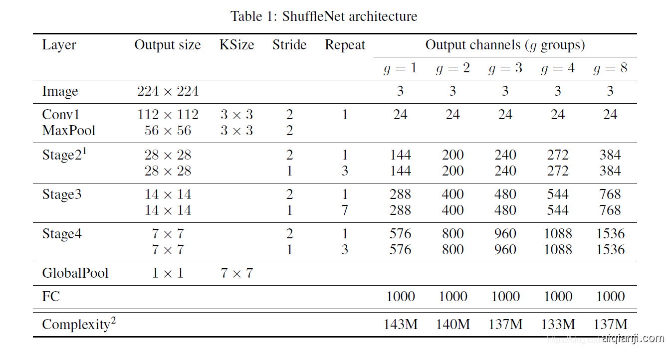
表1： ShuffleNet体系结构

Experiments 实验

We mainly evaluate our models on the ImageNet 2012 classification dataset. We follow most of the training settings and hyper-parameters used in , with two exceptions: (i) we set the weight decay to 4e-5 instead of 1e-4 and use linear-decay learning rate policy (decreased from 0.5 to 0); (ii) we use slightly less aggressive scale augmentation for data preprocessing. Similar modifications are also referenced in because such small networks usually suffer from underfitting rather than overfitting. It takes 1 or 2 days to train a model for $ 3\times 10^5 $ iterations on 4 GPUs, whose batch size is set to 1024. To benchmark, we compare single crop top-1 performance on ImageNet validation set, i.e. cropping $ 224\times 224 $ center view from $ 256\times $ input image and evaluating classification accuracy. We use exactly the same settings for all models to ensure fair comparisons.

我们主要评估对ImageNet 2016分类数据集上的模型 [ 26，4 ]。我们使用自己开发的系统进行训练，并遵循[ 37 ]中使用的大多数训练设置和超参数 ，但有两个例外：（i）将权重衰减设置为4e-5而不是1e-4，并使用线性衰减学习率策略（从0.5减少到0）；（ii）我们在数据预处理中使用略微不那么激进的积极扩展。在[ 12 ]中也引用了类似的修改， 因为这样的小型网络通常遭受欠拟合而不是过度拟合的困扰。在4个GPU上训$ 3\times 10^5 $迭代 需要1或2天，其批量大小设置为1024.
为了进行基准测试，我们在ImageNet验证集上比较了top-1的性能，即裁剪224×224 的中心视图 256× 输入图像并评估分类准确性。我们对所有模型的设置完全相同的设置以确保公平比较。

Ablation Study 消融研究

The core idea of ShuffleNet lies in pointwise group convolution and channel shuffle operation. In this subsection we evaluate them respectively.

ShuffleNet的核心思想在于第3.1节和第 3.2节中引用的逐点分组卷积和通道混洗操作 。在本小节中，我们分别对其进行评估。

Pointwise Group Convolutions 逐点分组卷积

To evaluate the importance of pointwise group convolutions, we compare ShuffleNet models of the same complexity whose numbers of groups range from 1 to 8. If the group number equals 1, no pointwise group convolution is involved and then the ShuffleNet unit becomes an "Xception-like" structure. For better understanding, we also scale the width of the networks to 3 different complexities and compare their classification performance respectively. Results are shown in Tablegroupconv.

我们比较了复杂度相同的ShuffleNet模型，其群数范围为1到8。如果群数等于1，则不涉及逐点群卷积，然后ShuffleNet单元变为“ Xception-像“ [ 3 ]结构。为了更好地理解，我们还将网络的宽度缩放到3个不同的复杂度，并分别比较它们的分类性能。结果示于表 2。

From the results, we see that models with group convolutions ( $ g>1 $ ) consistently perform better than the counterparts without pointwise group convolutions ( $ g=1 $ ). Smaller models tend to benefit more from groups. For example, for ShuffleNet 1 $ \times $ the best entry ( $ g=8 $ ) is 1.2% better than the counterpart, while for ShuffleNet 0.5 $ \times $ and 0.25 $ \times $ the gaps become 3.5% and 4.4% respectively. Note that group convolution allows more feature map channels for a given complexity constraint, so we hypothesize that the performance gain comes from wider feature maps which help to encode more information. In addition, a smaller network involves thinner feature maps, meaning it benefits more from enlarged feature maps.

从结果中，我们看到具有分组卷积的模型（G>1个）始终比没有逐点分组卷积（G=1个）要好。较小的模型往往会受益更多。例如，对于ShuffleNet 1× 最佳条目（G=3）比同类产品好1.0％，而ShuffleNet 0.5× 和0.25×差距分别变为2.4％和3.0％。请注意，对于给定的复杂性约束，分组卷积允许更多的特征图通道，因此我们假设性能增益来自有助于编码更多信息的更宽的特征图。此外，较小的网络涉及较薄的特征图，这意味着它从扩展的特征图中受益更多。

Table groupconv also shows that for some models (e.g. ShuffleNet 0.5 $ \times $ ) when group numbers become relatively large (e.g. $ g=8 $ ), the classification score saturates or even drops. With an increase in group number (thus wider feature maps), input channels for each convolutional filter become fewer, which may harm representation capability. Interestingly, we also notice that for smaller models such as ShuffleNet 0.25 $ \times $ larger group numbers tend to better results consistently, which suggests wider feature maps bring more benefits for smaller models.

表2还显示了对于某些模型（例如ShuffleNet 1×），当组号变得相对较大时（例如 G=4 或者 8），则分类得分达到饱和甚至下降。随着组数的增加（因此，特征图会更宽），每个卷积滤波器的输入通道会越来越少，这可能会损害表示能力。有趣的是，我们还注意到，对于较小的模型，例如ShuffleNet 0.25×较大的组数趋于一致地获得更好的结果，这表明较宽的特征图对于较小的模型尤为重要。受此启发，对于低成本模型，我们对表1中的体系结构进行了少许修改 ：我们在Stage3中删除了两个单元，并加宽了每个功能图，以保持整体复杂性。表2中显示了新体系结构（名为“ arch2 ”）的结果 。显然，新设计的模型始终优于同类模型。此外，逐点群卷积在体系结构中仍然有效。

Channel Shuffle vs. No Shuffle 通道混洗与无混洗操作

The purpose of shuffle operation is to enable cross-group information flow for multiple group convolution layers. Tableshuffle compares the performance of ShuffleNet structures (group number is set to 3 or 8 for instance) with/without channel shuffle. The evaluations are performed under three different scales of complexity. It is clear that channel shuffle consistently boosts classification scores for different settings. Especially, when group number is relatively large (e.g. $ g=8 $ ), models with channel shuffle outperform the counterparts by a significant margin, which shows the importance of cross-group information interchange.

通道混洗的目的是为多个组卷积层启用跨组信息流。表 3比较了带/不带通道混洗的ShuffleNet结构（例如，组号设置为3或8）的性能。评估是在三种不同的复杂度范围内进行的。显然，通道混洗可以持续提高不同设置的分类得分。特别是当组数较大时（例如G=8），带有通道混洗的模型要比同类模型大得多，这表明了跨组信息交换的重要性。

表3：带有/不带有通道随机播放的ShuffleNet（较小的数字表示更好的性能）

Comparison with Other Structure Units 与其他结构单元的比较

Recent leading convolutional units in VGG, ResNet, GoogleNet, ResNeXt and Xception have pursued state-of-the-art results with large models (e.g. $ \ge 1 $ GFLOPs), but do not fully explore low-complexity conditions. In this section we survey a variety of building blocks and make comparisons with ShuffleNet under the same complexity constraint. For fair comparison, we use the overall network architecture as shown in Tablearch. We replace the ShuffleNet units in Stage 2-4 with other structures, then adapt the number of channels to ensure the complexity remains unchanged. The structures we explored include: - \emph{VGG-like}. Following the design principle of VGG net, we use a two-layer 3 \times 3 convolutions as the basic building block. Different from , we add a Batch Normalization layer after each of the convolutions to make end-to-end training easier. - \emph{ResNet}. We adopt the "bottleneck" design in our experiment, which has been demonstrated more efficient in . Same as , the \emph{bottleneck ratio}\footnote{In the bottleneck-like units (like ResNet, ResNeXt or ShuffleNet) \emph{bottleneck ratio} implies the ratio of bottleneck channels to output channels. For example, bottleneck ratio = 1:4 means the output feature map is 4 times the width of the bottleneck feature map. } is also 1:4 . - \emph{Xception-like}. The original structure proposed in involves fancy designs or hyper-parameters for different stages, which we find difficult for fair comparison on small models. Instead, we remove the pointwise group convolutions and channel shuffle operation from ShuffleNet (also equivalent to ShuffleNet with g=1 ). The derived structure shares the same idea of depthwise separable convolution" as in , which is called an \emph{Xception-like} structure here. - \emph{ResNeXt}. We use the settings of \emph{cardinality} =16 and bottleneck ratio =1:2 as suggested in . We also explore other settings, e.

与其他结构单位的比较

VGG [ 27 ]，ResNet [ 9 ]，GoogleNet [ 30 ]，ResNeXt [ 37 ]和Xception [ 3 ]中最近的领先卷积单元 都采用大型模型（例如，≥1个GFLOPs），但不能完全探索低复杂性条件。在本节中，我们将调查各种构建基块，并在相同的复杂性约束下与ShuffleNet进行比较。

为了公平地比较，我们使用表1中所示的总体网络体系结构 。我们将Stage 2-4中的ShuffleNet单元替换为其他结构，然后调整通道数以确保复杂度保持不变。我们探索的结构包括：

• 像VGG一样。遵循VGG net [ 27 ]的设计原理 ，我们使用两层3×3个卷积作为基本构建块。与[ 27 ]不同 ，我们在每个卷积之后添加了一个批处理归一化层 [ 14 ]，以简化端到端的训练。
• ResNet。我们在实验中采用了“瓶颈”设计，这在[ 9 ]中得到了更有效的证明 。与[ 9 ]相同 ，瓶颈比率为 =1:4
• 类似Xception。在[ 3 ]中提出的原始结构 涉及不同阶段的精美设计或超参数，我们发现很难在小模型上进行公平比较。取而代之的是，我们从ShuffleNet（也等效于ShuffleNetG=1个）。派生的结构与[ 3 ]中的“深度可分离卷积”具有相同的思想，在 此称为Xception-like结构。
• ResNeXt。我们使用基数的设置** =16 和瓶颈比率 =1个：2个如[ 37 ]中建议的 。我们还将探索其他设置，例如瓶颈比率=1：4，并获得相似的结果。

We use exactly the same settings to train these models. Results are shown in Tablestructues. Our ShuffleNet models outperform most others by a significant margin under different complexities. Interestingly, we find an empirical relationship between feature map channels and classification accuracy. For example, under the complexity of 38 MFLOPs, output channels of Stage 4 (see Tablearch) for VGG-like, ResNet, ResNeXt, Xception-like, ShuffleNet models are 50, 192, 192, 288, 576 respectively, which is consistent with the increase of accuracy. Since the efficient design of ShuffleNet, we can use more channels for a given computation budget, thus usually resulting in better performance. Note that the above comparisons do not include GoogleNet or Inception series. We find it nontrivial to generate such Inception structures to small networks because the original design of Inception module involves too many hyper-parameters. As a reference, the first GoogleNet version has 31.3% top-1 error at the cost of 1.5 GFLOPs (See Tablecomplexity). More sophisticated Inception versions are more accurate, however, involve significantly increased complexity. Recently, Kim et al. propose a lightweight network structure named PVANET which adopts Inception units. Our reimplemented PVANET (with 224 $ \times $ 224 input size) has 29.7% classification error with a computation complexity of 557 MFLOPs, while our ShuffleNet 2x model ( $ g=3 $ ) gets 26.3% with 524 MFLOPs (see Tablecomplexity).

我们使用完全相同的设置来训练这些模型。结果示于表 4。在不同的复杂性下，我们的ShuffleNet模型要比其他大多数模型好得多。有趣的是，我们发现了特征图通道与分类精度之间的经验关系。例如，在38个MFLOP的复杂性下，类VGG，ResNet，ResNeXt，类Xception，ShuffleNet模型的第4阶段（请参见表1）的输出通道分别为 50、192、192、288、576，这是一致的随着准确性的提高。由于ShuffleNet的高效设计，对于给定的计算预算，我们可以使用更多的通道，因此通常可以获得更好的性能。

表 4还在较浅但较宽的体系结构上评估了各种模型（标记为“ arch2 ”，有关详细信息，请参见4.1.1）。可以看出，与其他结构相比，ShuffleNet仍然取得了出色的结果。

请注意，上述比较不包括googlenet 或 inception 系列。我们发现将这样的Inception结构生成到小型网络并非易事，因为Inception模块的原始设计涉及太多的超参数。作为参考，Kim等。最近已经提出了一种轻量级的网络结构，称为*PVANET * [ 18 ]，它采用了Inception单元。我们重新实现的PVANET（带有224×224个输入大小）具有35.3％的分类错误，计算复杂度为557个MFLOP，而我们的ShuffleNet 2x模型（G=3）以524个MFLOP获得29.1％（请参见表 6）。因此，即使缺乏直接比较，Inception在琐碎的环境中也不可能超过ShuffleNet。

Comparison with MobileNets and Other Frameworks 与MOBILENETS和其他框架的比较

Recently Howard et al. have proposed MobileNets which mainly focus on efficient network architecture for mobile devices. MobileNet takes the idea of depthwise separable convolution from and achieves state-of-the-art results on small models. Tablemobilecls compares classification scores under a variety of complexity levels. It is clear that our ShuffleNet models are superior to MobileNet for all the complexities. Though our ShuffleNet network is specially designed for small models ( $ <150 $ MFLOPs), we find it is still better than MobileNet for higher computation cost, e.g. 3.1% more accurate than MobileNet 1 $ \times $ at the cost of 500 MFLOPs. For smaller networks ( $ \sim $ 40 MFLOPs) ShuffleNet surpasses MobileNet by . Note that our ShuffleNet architecture contains 50 layers while MobileNet only has 28 layers. For better understanding, we also try ShuffleNet on a 26-layer architecture by removing half of the blocks in Stage 2-4 (see "ShuffleNet 0.5 $ \times $ shallow ( $ g=3 $ )" in Tablemobilecls). Results show that the shallower model is still significantly better than the corresponding MobileNet, which implies that the effectiveness of ShuffleNet mainly results from its efficient structure, not the depth. Tablecomplexity compares our ShuffleNet with a few popular models. Results show that with similar accuracy ShuffleNet is much more efficient than others. For example, ShuffleNet 0.5 $ \times $ is theoretically 18 $ \times $ faster than AlexNet with comparable classification score. We will evaluate the actual running time in Sec actual. It is also worth noting that the simple architecture design makes it easy to equip ShuffeNets with the latest advances such as . For example, in the authors propose Squeeze-and-Excitation (SE) blocks which achieve state-of-the-art results on large ImageNet models. We find SE modules also take effect in combination with the backbone ShuffleNets, for instance, boosting the top-1 error of ShuffleNet 2 $ \times $ to 24.7%(shown in Tablemobilecls). Interestingly, though negligible increase of theoretical complexity, we find ShuffleNets with SE modules are usually $ 25 \sim 40% $ slower than the raw ShuffleNets on mobile devices, which implies that actual speedup evaluation is critical on low-cost architecture design. In Secactual we will make further discussion.

最近howard等。已提出Mobilenets，主要关注移动设备的有效网络架构。 MobileNet从小模型来实现深度可分离卷积的想法，从而实现了最先进的结果。

表 5比较了各种复杂性级别下的分类得分。显然，我们的ShuffleNet模型在所有复杂性方面都优于MobileNet。尽管我们的ShuffleNet网络是专门为小型机型设计的（<150MFLOPs），我们发现它在计算成本上仍比MobileNet稍好。对于较小的网络（约40个MFLOP），ShuffleNet超过MobileNet 6.7％。请注意，我们的ShuffleNet架构包含50层（或arch2则为44层），而MobileNet仅包含28层。为了更好地理解，我们还通过在阶段2-4中删除一半的块来尝试在26层体系结构上使用ShuffleNet（请参阅“ ShuffleNet 0.5× （G=3）”表 5）。结果表明，该浅模型仍然显著优于相应MobileNet，这意味着的ShuffleNet的有效性，主要是由于从它的有效的结构，而不是深度。

表 6将我们的ShuffleNet与一些流行的模型进行了比较。结果表明，以相似的精度ShuffleNet比其他的效率更高。例如，ShuffleNet 0.5× 理论上是18×速度比具有类似分类评分的AlexNet [ 19 ]快 。我们将在4.5节中评估实际的运行时间。

Generalization Ability 泛化能力

To evaluate the generalization ability for transfer learning, we test our ShuffleNet model on the task of MS COCO object detection. We adopt Faster-RCNN as the detection framework and use the publicly released Caffe code for training with default settings. Similar to , the models are trained on the COCO train+val dataset excluding 5000 minival images and we conduct testing on the minival set. Tabledet shows the comparison of results trained and evaluated on two input resolutions. Comparing ShuffleNet 2 $ \times $ with MobileNet whose complexity are comparable (524 vs. 569 MFLOPs), our ShuffleNet 2 $ \times $ surpasses MobileNet by a significant margin on both resolutions; our ShuffleNet 1 $ \times $ also achieves comparable results with MobileNet on 600 $ \times $ resolution, but has $ \sim $ 4 $ \times $ complexity reduction. We conjecture that this significant gain is partly due to ShuffleNet's simple design of architecture without bells and whistles.

为了评估迁移学习的泛化能力，我们在MS COCO对象检测任务中测试了ShuffleNet模型 [ 21 ]。我们采用更快RCNN [ 25 ]作为检测框架和使用公开发布来自Caffe代码 [ 25，16 ]接受培训的默认设置。与[ 12 ]相似 ，模型在不包含5000个最小图像的COCO train + val数据集上进行训练，我们对最小集合进行测试。表 7显示了在两种输入分辨率下训练和评估的结果的比较。比较ShuffleNet 2× 与ShuffleNet 2相比，MobileNet的复杂度可比（524 vs. 569 MFLOP）×两项决议均大大超过MobileNet；我们的ShuffleNet 1× 在600上通过MobileNet也获得可比的结果× 分辨率，但具有〜4×降低复杂性。我们推测，这一巨大的收益部分是由于ShuffleNet的架构设计简单而没有花哨。

Actual Speedup Evaluation 实际加速评估

Finally, we evaluate the actual inference speed of ShuffleNet models on a mobile device with an ARM platform. Though ShuffleNets with larger group numbers (e.g. $ g=4 $ or $ g=8 $ ) usually have better performance, we find it less efficient in our current implementation. Empirically $ g=3 $ usually has a proper trade-off between accuracy and actual inference time. As shown in Tableactual, three input resolutions are exploited for the test. Due to memory access and other overheads, we find every 4 $ \times $ theoretical complexity reduction usually results in $ \sim $ 2.6 $ \times $ actual speedup in our implementation. Nevertheless, compared with AlexNet our ShuffleNet 0.5 $ \times $ model still achieves $ \sim $ 13 $ \times $ speedup under comparable classification accuracy (the theoretical speedup is 18 $ \times $ ), which is much faster than previous AlexNet-level models or speedup approaches such as .

最后，我们评估具有ARM平台的移动设备上ShuffleNet模型的实际推理速度。如表8所示， 测试使用了三种输入分辨率。由于内存访问和其他开销，我们发现每4个× 理论上的复杂度降低通常导致〜2.6×我们实施中的实际加速。尽管如此，与AlexNet [ 19 ]相比， 我们的ShuffleNet 0.5× 模型仍然达到〜13× 在可比的分类精度下的实际加速比（理论加速比为18×），它比以前的AlexNet级模型或加速快得多的方法，例如 [ 13，15，20，38，39，35 ]。