.
MobileNets: Efficient Convolutional Neural Networks for Mobile Vision Applications 用于移动视觉应用的高效卷积神经网络
校正者:
布丁
中英文论文对照合集 https://aiqianji.com/blog/articles
Abstract
We present a class of efficient models called MobileNets for mobile and embedded vision applications. MobileNets are based on a streamlined architecture that uses depthwise separable convolutions to build light weight deep neural networks. We introduce two simple global hyper-parameters that efficiently trade off between latency and accuracy. These hyper-parameters allow the model builder to choose the right sized model for their application based on the constraints of the problem. We present extensive experiments on resource and accuracy tradeoffs and show strong performance compared to other popular models on ImageNet classification. We then demonstrate the effectiveness of MobileNets across a wide range of applications and use cases including object detection, finegrain classification, face attributes and large scale geo-localization.
摘要
本文针对嵌入式视觉应用领域,提出一个新颖的MobileNets网络,该网络使用了深度可分离卷积来构建轻量级深度神经网络。我们介绍了两个简单的全局超参数,使得模型可以在速度和准确度之间有效地进行折中。这些超参数允许模型构建器根据问题的约束,为其应用程序选择正确的大小模型。我们对资源和准确性权衡提供了广泛的实验,并与Imagenet分类的其他流行模型相比表现出优异的表现。然后,我们展示了Mobilenets跨各种应用程序的有效性和用例,包括物体检测,FineGrain分类,面部属性和大规模地理定位。
Introduction 简介
Convolutional neural networks have become ubiquitous in computer vision ever since AlexNet popularized deep convolutional neural networks by winning the ImageNet Challenge: ILSVRC 2012 . The general trend has been to make deeper and more complicated networks in order to achieve higher accuracy . However, these advances to improve accuracy are not necessarily making networks more efficient with respect to size and speed. In many real world applications such as robotics, self-driving car and augmented reality, the recognition tasks need to be carried out in a timely fashion on a computationally limited platform.
卷积神经网络在计算机视觉中普遍存在,自AlexNet通过赢得ImageNet挑战赢得了深度卷积神经网络:ILSVRC 2012。一般趋势一直是制造更深刻更复杂的网络,以实现更高的准确性。然而,这些提高准确性的进步不一定使网络在尺寸和速度方面更有效。在许多现实世界的应用程序中,如机器人,自驾驶汽车和增强现实,需要在计算有限的平台上以及时的方式进行识别任务。
This paper describes an efficient network architecture and a set of two hyper-parameters in order to build very small, low latency models that can be easily matched to the design requirements for mobile and embedded vision applications. Section prior reviews prior work in building small models. Section mobilenet describes the MobileNet architecture and two hyper-parameters width multiplier and resolution multiplier to define smaller and more efficient MobileNets. Section exp describes experiments on ImageNet as well a variety of different applications and use cases. Section conclusion closes with a summary and conclusion.
本文介绍了一种有效的网络架构和两个超参数,以便构建非常小的低延迟模型,可以轻松匹配移动和嵌入式视觉应用程序的设计要求。第一部分回顾了小模型建立的先前工作。 MobileNet部分描述了MobileNet架构和两个超参数:宽度乘法器和分辨率乘法器,以定义更小且更高效的移动单元。 exp章节描述了Imagenet的实验以及各种不同的应用和用例。最后是总结部分

图1: MobileNet模型可以应用于各种识别任务,以实现设备智能的高效。
Prior Work 相关工作
There has been rising interest in building small and efficient neural networks in the recent literature, e.g. . Many different approaches can be generally categorized into either compressing pretrained networks or training small networks directly. This paper proposes a class of network architectures that allows a model developer to specifically choose a small network that matches the resource restrictions (latency, size) for their application. MobileNets primarily focus on optimizing for latency but also yield small networks. Many papers on small networks focus only on size but do not consider speed.
在最近的文献中构建小型高效的神经网络的兴趣正在增长,例如[ 16,34,12,36,22 ]。通常这些不同的方法归类为压缩预训练网络和直接训练小型网络。本文提出了一类网络体系结构,允许模型开发人员专门为其应用选择与资源限制(延迟,大小)相匹配的小型网络。MobileNets主要专注于优化速度,但也会产生小型网络。关于小型网络的许多论文只关注规模,却不考虑速度。
MobileNets are built primarily from depthwise separable convolutions initially introduced in and subsequently used in Inception models to reduce the computation in the first few layers. Flattened networks build a network out of fully factorized convolutions and showed the potential of extremely factorized networks. Independent of this current paper, Factorized Networks introduces a similar factorized convolution as well as the use of topological connections. Subsequently, the Xception network demonstrated how to scale up depthwise separable filters to out perform Inception V3 networks. Another small network is Squeezenet which uses a bottleneck approach to design a very small network. Other reduced computation networks include structured transform networks and deep fried convnets . A different approach for obtaining small networks is shrinking, factorizing or compressing pretrained networks. Compression based on product quantization , hashing , and pruning, vector quantization and Huffman coding have been proposed in the literature. Additionally various factorizations have been proposed to speed up pretrained networks . Another method for training small networks is distillation which uses a larger network to teach a smaller network. It is complementary to our approach and is covered in some of our use cases in section exp. Another emerging approach is low bit networks .
MobileNets主要是由[ 26 ]中最初引入并随后用于Inception模型[ 13 ]中的深度可分离卷积构建的,以减少前几层的计算量。 Flattened networks [ 16 ]由完全分解的卷积构建网络,并显示了高度分解的网络的潜力。独立于本文, Factorized Networks [ 34 ]引入了类似的分解卷积以及拓扑连接的使用。随后,Xception网络[ 3 ]演示了如何按比例放大深度可分离滤波器,以执行Inception V3网络。另一个小型网络是Squeezenet [ 12 ],它使用瓶颈方法设计了一个非常小的网络。其他减少的计算网络包括结构化转换网络[ 28 ]和deep fried convnets[ 37 ]。
获得小型网络的另一种方法是收缩,分解或压缩预训练的网络。在文献中已经提出了基于乘积量化[ 36 ],散列[ 2 ]以及修剪,矢量量化和霍夫曼编码[ 5 ]的压缩。此外各种因式分解已被提出以加快预训练网络[ 14,20 ]。训练小型网络的另一种方法是蒸馏[ 9 ]它使用较大的网络来教授较小的网络。它是对我们方法的补充,并且在第4节中的一些用例中进行了介绍。另一个新兴方法是低比特网络[ 4,22,11 ]。
MobileNet Architecture MOBILENET体系结构
In this section we first describe the core layers that MobileNet is built on which are depthwise separable filters. We then describe the MobileNet network structure and conclude with descriptions of the two model shrinking hyper-parameters width multiplier and resolution multiplier.
在本节中,我们首先描述了MobileNet构建的核心层,它是深度可分离的滤波器。然后,我们描述了MobileNet网络结构并结论,描述了两个模型缩小的超参数:宽度乘数和分辨率乘法器。
Depthwise Separable Convolution 深度可分离卷积
The MobileNet model is based on depthwise separable convolutions which is a form of factorized convolutions which factorize a standard convolution into a depthwise convolution and a $ 1 \times 1 $ convolution called a pointwise convolution.
MobileNet模型基于深度可分离卷积,该卷曲是一种分解卷积的形式,其将标准卷积分解为深度卷积和$ 1 \times 1 $卷积,称为点卷积。对于MobiLenets,深度卷积将单个过滤器应用于每个输入通道。然后,点卷积然后应用$ 1 \times 1 $卷积以组合输出的深度卷积。
For MobileNets the depthwise convolution applies a single filter to each input channel. The pointwise convolution then applies a $ 1 \times 1 $ convolution to combine the outputs the depthwise convolution. A standard convolution both filters and combines inputs into a new set of outputs in one step. The depthwise separable convolution splits this into two layers, a separate layer for filtering and a separate layer for combining. This factorization has the effect of drastically reducing computation and model size.Figure dw_conv shows how a standard convolution dw_conv_a is factorized into a depthwise convolution dw_conv_b and a $ 1 \times 1 $ pointwise convolution dw_conv_c.
标准卷积在一个步骤中,两个滤波器将输入组合成一组新的输出。深度可分离卷积将其分成两层,是用于独立的滤波器和独立的组合层。这种分解具有大幅减少计算和模型大小的效果。图2显示了如何将标准卷积2(a)分解为深度卷积2(b)和1×1个点向卷积2(c)。


A standard convolutional layer takes as input a $ D_F \times D_F \times M $ feature map $ F $ and produces a $ D_F \times D_F \times N $ feature map $ G $ where $ D_F $ is the spatial width and height of a square input feature map We assume that the output feature map has the same spatial dimensions as the input and both feature maps are square. Our model shrinking results generalize to feature maps with arbitrary sizes and aspect ratios. , $ M $ is the number of input channels (input depth), $ D_G $ is the spatial width and height of a square output feature map and $ N $ is the number of output channel (output depth). The standard convolutional layer is parameterized by convolution kernel $ K $ of size $ D_K \times D_K \times M \times N $ where $ D_K $ is the spatial dimension of the kernel assumed to be square and $ M $ is number of input channels and $ N $ is the number of output channels as defined previously. The output feature map for standard convolution assuming stride one and padding is computed as:
输入的特征映射$ F 尺寸为$ $ D_F \times D_F \times M $,输出的特征图$ G $ 尺寸为 $ D_F \times D_F \times N $ ,其中$ D_F $是正方形输入特征图的空间宽度和高度。(我们假设输出特征图具有与输入相同的空间尺寸,并且两个特征图均为正方形。我们的模型缩小结果可以概括为具有任意大小和纵横比的特征图。)$ M $是输入通道的数量(输入深度),$ D_G $是方形输出特征图的空间宽度和高度,$ N $是输出通道(输出深度)的数量。标准卷积层通过卷积核$ K $参数化$ D_K \times D_K \times M \times N $其中$ D_K $是假定为正方形的内核的空间尺寸,$ M $是输入通道的数量和$ N $是先前定义的输出通道数。
假设跨度为1和填充为标准卷积的输出特征图,计算公式为:
$$ G_{k,l,n} = \sum_{i,j,m} K_{i,j,m,n}\cdot F_{k+i-1,l+j-1,m} $$
Standard convolutions have the computational cost of: 标准卷积的计算成本为:
$$ D_K \cdot D_K \cdot M \cdot N \cdot D_F \cdot D_F $$
where the computational cost depends multiplicatively on the number of input channels $ M $ , the number of output channels $ N $ the kernel size $ D_k \times D_k $ and the feature map size $ D_F \times D_F $ . MobileNet models address each of these terms and their interactions. First it uses depthwise separable convolutions to break the interaction between the number of output channels and the size of the kernel. The standard convolution operation has the effect of filtering features based on the convolutional kernels and combining features in order to produce a new representation.
,其中计算成本差异依赖在输入通道$ M $的数量上,输出通道的数量$ N $内核大小$ D_k \times D_k $和特征映射大小$ D_F \times D_F $。 MobileNet模型解决了这些相互关系。首先,它使用深度可分离的卷积来破坏输出通道数与内核的大小之间的交互。标准卷积操作基于卷积核和组合特征的滤波功能效果,以产生新的表示。
The filtering and combination steps can be split into two steps via the use of factorized convolutions called depthwise separable convolutions for substantial reduction in computational cost. Depthwise separable convolution are made up of two layers: depthwise convolutions and pointwise convolutions. We use depthwise convolutions to apply a single filter per each input channel (input depth). Pointwise convolution, a simple $ 1 \times 1 $ convolution, is then used to create a linear combination of the output of the depthwise layer. MobileNets use both batchnorm and ReLU nonlinearities for both layers. Depthwise convolution with one filter per input channel (input depth) can be written as:
滤波和组合步骤可以通过使用称为深度可分离卷积的分解卷积分为两个步骤,以大幅降低计算成本。深度可分离卷积由两层组成:深度卷积和点卷积。我们使用深度卷积在每个输入通道(输入深度)上应用单个滤波器。点卷积,简单1×1个卷积,然后用于创建深度层输出的线性组合。MobileNets对这两个层都使用了batchnorm和ReLU非线性。
每个输入通道(输入深度)带有一个滤波器的深度卷积可以写成
$$ \hat{G}{k,l,m} = \sum{i,j} \hat{K}{i,j,m} \cdot F{k+i-1,l+j-1,m} $$
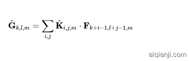
where $ \hat{K} $ is the depthwise convolutional kernel of size $ D_K \times D_K \times M $ where the $ m_{th} $ filter in $ \hat{K} $ is applied to the $ m_{th} $ channel in $ F $ to produce the $ m_{th} $ channel of the filtered output feature map $ \hat{G} $ . Depthwise convolution has a computational cost of:
,其中$\hat{K} $是$ D_K \times D_K \times M $的深度卷积核,其中$中的$ m_{th} $滤波器T91_0 $应用于$ F $中的$ m_{th} $通道,以生成滤波输出功能映射$\hat{G} $的$ m_{th} $通道。深度卷积具有以下计算成本:
$$ D_K \cdot D_K \cdot M \cdot D_F \cdot D_F $$
Depthwise convolution is extremely efficient relative to standard convolution. However it only filters input channels, it does not combine them to create new features. So an additional layer that computes a linear combination of the output of depthwise convolution via $ 1 \times 1 $ convolution is needed in order to generate these new features. The combination of depthwise convolution and $ 1\times1 $ (pointwise) convolution is called depthwise separable convolution which was originally introduced in . Depthwise separable convolutions cost:
深度卷积相对于标准卷积非常有效。但是它只对输入通道进行滤波,它不会组合它们以创建新功能。因此,需要一种附加层,其通过$ 1 \times 1 $卷积需要计算深度卷积的输出的线性组合,以便生成这些新功能。
深度卷积和 1×1个(逐点)卷积称为“深度可分离卷积”,最初是在[ 26 ]中引入的。
深度可分离卷积代价:
$$ D_K \cdot D_K \cdot M \cdot D_F \cdot D_F + M \cdot N \cdot D_F \cdot D_F $$
which is the sum of the depthwise and $ 1 \times 1 $ pointwise convolutions. By expressing convolution as a two step process of filtering and combining we get a reduction in computation of: MobileNet uses $ 3 \times 3 $ depthwise separable convolutions which uses between 8 to 9 times less computation than standard convolutions at only a small reduction in accuracy as seen in Section exp.
,它是深度和$ 1 \times 1 $点卷积的总和。通过表达卷积作为过滤和组合的两个步骤过程,我们得到了计算的减少:MobileNet使用$ 3 \times 3 $深度可分离卷曲,其使用的计算比标准卷曲更小的准确性,所以计算得多。在exp节中看到。
Additional factorization in spatial dimension such as in does not save much additional computation as very little computation is spent in depthwise convolutions.
在空间维度附加因式分解,如在[ 16,31 ]不保存多少额外的计算,因为在深度卷积中花费了很少的计算。

Network Structure and Training 网络结构与训练
The MobileNet structure is built on depthwise separable convolutions as mentioned in the previous section except for the first layer which is a full convolution. By defining the network in such simple terms we are able to easily explore network topologies to find a good network. The MobileNet architecture is defined in Table 1. All layers are followed by a batchnorm [13] and ReLU nonlinearity with the exception of the final fully connected layer which has no nonlinearity and feeds into a softmax layer for classification. Figure 3 contrasts a layer with regular convolutions, batchnorm and ReLU nonlinearity to the factorized layer with depthwise convolution, 1×1 pointwise convolution as well as batchnorm and ReLU after each convolutional layer. Down sampling is handled with strided convolution in the depthwise convolutions as well as in the first layer. A final average pooling reduces the spatial resolution to 1 before the fully connected layer. Counting depthwise and pointwise convolutions as separate layers, MobileNet has 28 layers.
如前一节所述,MobileNet结构建立在深度可分离卷积之上,第一层是完整卷积。通过以这种简单的术语定义网络,我们可以轻松地探索网络拓扑以找到一个好的网络。表1中定义了MobileNet体系结构。除了最后的完全连接的层(没有非线性,并馈入softmax层进行分类)外,所有层都遵循batchnorm [ 13 ]和ReLU非线性。图3将具有规则卷积,batchnorm和ReLU非线性的层与具有深度卷积的分解层进行了对比,1个×1个每个卷积层之后的逐点卷积以及batchnorm和ReLU。下采样是在深度卷积以及第一层中通过跨步卷积来处理的。最终平均池在完全连接的层之前将空间分辨率降低为1。将深度卷积和点积卷积计为单独的层,MobileNet有28层。
It is not enough to simply define networks in terms of a small number of Mult-Adds. It is also important to make sure these operations can be efficiently implementable. For instance unstructured sparse matrix operations are not typically faster than dense matrix operations until a very high level of sparsity. Our model structure puts nearly all of the computation into dense 1×1 convolutions. This can be implemented with highly optimized general matrix multiply (GEMM) functions. Often convolutions are implemented by a GEMM but require an initial reordering in memory called im2col in order to map it to a GEMM. For instance, this approach is used in the popular Caffe package [15]. 1×1 convolutions do not require this reordering in memory and can be implemented directly with GEMM which is one of the most optimized numerical linear algebra algorithms. MobileNet spends 95% of it’s computation time in 1×1 convolutions which also has 75% of the parameters as can be seen in Table 2. Nearly all of the additional parameters are in the fully connected layer.
仅用少量的Mult-Adds定义网络是不够的。确保这些操作可以有效实施也很重要。例如,直到非常高的稀疏性,非结构化稀疏矩阵运算通常不比密集矩阵运算快。我们的模型结构使几乎所有计算都变得密集1个×1个卷积。这可以通过高度优化的通用矩阵乘法(GEMM)函数来实现。卷积通常由GEMM实现,但需要在内存中进行名为im2col的初始重新排序,才能将其映射到GEMM。例如,这种方法在流行的Caffe包中使用[ 15 ]。1个×1个卷积不需要在内存中进行这种重新排序,可以直接使用GEMM进行实现,GEMM是最优化的数值线性代数算法之一。MobileNet支出95% 它的计算时间 1个×1个 卷积也有 75%表2中可以看到这些参数。几乎所有其他参数都在完全连接的层中。
MobileNet models were trained in TensorFlow [1] using RMSprop [33] with asynchronous gradient descent similar to Inception V3 [31]. However, contrary to training large models we use less regularization and data augmentation techniques because small models have less trouble with overfitting. When training MobileNets we do not use side heads or label smoothing and additionally reduce the amount image of distortions by limiting the size of small crops that are used in large Inception training [31]. Additionally, we found that it was important to put very little or no weight decay (l2 regularization) on the depthwise filters since their are so few parameters in them. For the ImageNet benchmarks in the next section all models were trained with same training parameters regardless of the size of the model.
MobileNet模型在TensorFlow [ 1 ]中使用RMSprop [ 33 ]的异步梯度下降来训练,类似于Inception V3 [ 31 ]。但是,与训练大型模型相反,我们使用较少的正则化和数据增强技术,因为小型模型的过拟合麻烦较小。在训练MobileNets时,我们不使用侧边或标签平滑处理,并且通过限制在大型Inception训练中使用的小农作物的大小来减少失真的图像量[ 31 ]。此外,我们发现,对深度过滤器进行很少或没有权重衰减(l 2正则化)是很重要的,因为它们中的参数太少了。对于下一部分中的ImageNet基准,无论模型的大小如何,所有模型都使用相同的训练参数进行训练。
| Type / Stride | Filter Shape | Input Size |
|---|---|---|
| Conv / s2 | 3×3×3×32 | 224×224×3 |
| Conv dw / s1 | 3×3×32 dw | 112×112×32 |
| Conv / s1 | 1×1×32×64 | 112×112×32 |
| Conv dw / s2 | 3×3×64 dw | 112×112×64 |
| Conv / s1 | 1×1×64×128 | 56×56×64 |
| Conv dw / s1 | 3×3×128 dw | 56×56×128 |
| Conv / s1 | 1×1×128×128 | 56×56×128 |
| Conv dw / s2 | 3×3×128 dw | 56×56×128 |
| Conv / s1 | 1×1×128×256 | 28×28×128 |
| Conv dw / s1 | 3×3×256 dw | 28×28×256 |
| Conv / s1 | 1×1×256×256 | 28×28×256 |
| Conv dw / s2 | 3×3×256 dw | 28×28×256 |
| Conv / s1 | 1×1×256×512 | 14×14×256 |
| 5× Conv dw / s1 | 3×3×512 dw | 14×14×512 |
| Conv / s1 | 1×1×512×512 | 14×14×512 |
| Conv dw / s2 | 3×3×512 dw | 14×14×512 |
| Conv / s1 | 1×1×512×1024 | 7×7×512 |
| Conv dw / s2 | 3×3×1024 dw | 7×7×1024 |
| Conv / s1 | 1×1×1024×1024 | 7×7×1024 |
| Avg Pool / s1 | Pool 7×7 | 7×7×1024 |
| FC / s1 | 1024×1000 | 1×1×1024 |
| Softmax / s1 | Classifier | 1×1×1000 |
Table 1: MobileNet Body Architecture
表1: MobileNet主体架构

Figure 3: Left: Standard convolutional layer with batchnorm and ReLU. Right: Depthwise Separable convolutions with Depthwise and Pointwise layers followed by batchnorm and ReLU.
图3:左:具有batchnorm和ReLU的标准卷积层。右:Depthwise可拆分卷积,其中Depthwise和Pointwise层紧随其后是batchnorm和ReLU。
| Type | Mult-Adds | Parameters |
|---|---|---|
| Conv 1×1 | 94.86% | 74.59% |
| Conv DW 3×3 | 3.06% | 1.06% |
| Conv 3×3 | 1.19% | 0.02% |
| Fully Connected | 0.18% | 24.33% |
Table 2: Resource Per Layer Type 表2:每种层类型的资源
Width Multiplier: Thinner Models 宽度乘数:更薄的模型
Although the base MobileNet architecture is already small and low latency, many times a specific use case or application may require the model to be smaller and faster. In order to construct these smaller and less computationally expensive models we introduce a very simple parameter $ \alpha $ called width multiplier. The role of the width multiplier $ \alpha $ is to thin a network uniformly at each layer. For a given layer and width multiplier $ \alpha $ , the number of input channels $ M $ becomes $ \alpha M $ and the number of output channels $ N $ becomes $ \alpha N $ . The computational cost of a depthwise separable convolution with width multiplier $ \alpha $ is:
尽管基本的MobileNet体系结构已经很小并且延迟很短,但是很多时候,特定的用例或应用程序可能要求模型更小,更快。为了构造这些较小且计算量较小的模型,我们引入了一个非常简单的参数$\alpha $称为宽度乘法器。宽度乘法器$\alpha $的作用是在每层均匀地缩小网络。对于给定的层和宽度乘法器$\alpha $,输入通道$ M $的数量变为$\alpha M $和输出通道$ N $的数量变为$\alpha N $。具有宽度乘法器$\alpha $的深度可分离卷积的计算成本是:
$$ D_K \cdot D_K \cdot\alpha M \cdot D_F \cdot D_F + \alpha M \cdot\alpha N \cdot D_F \cdot D_F $$
where $ \alpha\in(0,1] $ with typical settings of 1, 0.75, 0.5 and 0.25. $ \alpha=1 $ is the baseline MobileNet and $ \alpha<1 $ are reduced MobileNets. Width multiplier has the effect of reducing computational cost and the number of parameters quadratically by roughly $ \alpha^2 $ . Width multiplier can be applied to any model structure to define a new smaller model with a reasonable accuracy, latency and size trade off. It is used to define a new reduced structure that needs to be trained from scratch.
其中$\alpha\in(0,1] $ 通常设置为1、0.75、0.5和0.25。 $\alpha=1 $是基线MOBILENET和$\alpha<1 $减少了MOBILENETS。宽度乘数通过大致$\alpha^2 $逐步降低计算成本和参数数量的效果。宽度乘法器可以应用于任何模型结构,以定义具有合理精度,延迟和尺寸折衷的新的较小模型。它用于定义需要从头开始训练的新的精简结构。
在哪里 α∈(0,1个] 通常设置为1、0.75、0.5和0.25。 α=1个 是baseline MobileNet 和 α<1个 reduced MobileNets。宽度乘数的作用是将计算量和参数数量大约减少了两倍α2个。宽度乘数可以应用于任何模型结构,以合理的精度,等待时间和尺寸折衷来定义新的较小模型。它用于定义新的精简结构,需要从头开始进行培训。
Resolution Multiplier: Reduced Representation 分辨率乘数:减少表达
The second hyper-parameter to reduce the computational cost of a neural network is a resolution multiplier $ \rho $ . We apply this to the input image and the internal representation of every layer is subsequently reduced by the same multiplier. In practice we implicitly set $ \rho $ by setting the input resolution. We can now express the computational cost for the core layers of our network as depthwise separable convolutions with width multiplier $ \alpha $ and resolution multiplier $ \rho $ :
减少神经网络计算成本的第二个超参数是分辨率乘数 ρ。我们将其应用于输入图像,然后通过相同的乘数来减少每一层的内部表示。在实践中,我们 通过设置输入分辨率隐式设置ρ。
现在,我们可以将网络核心层的计算成本表示为具有宽度乘数的深度可分离卷积 α 和分辨率乘数 ρ:
$$ D_K \cdot D_K \cdot\alpha M \cdot\rho D_F \cdot\rho D_F + \alpha M \cdot\alpha N \cdot\rho D_F \cdot\rho D_F $$
where $ \rho\in(0,1] $ which is typically set implicitly so that the input resolution of the network is 224, 192, 160 or 128. $ \rho=1 $ is the baseline MobileNet and $ \rho<1 $ are reduced computation MobileNets. Resolution multiplier has the effect of reducing computational cost by $ \rho^2 $ . As an example we can look at a typical layer in MobileNet and see how depthwise separable convolutions, width multiplier and resolution multiplier reduce the cost and parameters. Table layer_resource shows the computation and number of parameters for a layer as architecture shrinking methods are sequentially applied to the layer. The first row shows the Mult-Adds and parameters for a full convolutional layer with an input feature map of size $ 14 \times 14 \times 512 $ with a kernel $ K $ of size $ 3 \times 3 \times 512 \times 512 $ . We will look in detail in the next section at the trade offs between resources and accuracy.
其中$\rho\in(0,1] $通常隐含地设置,以便网络的输入分辨率为224,192,160或128. $\rho=1 $是baseline MobileNet 和$\rho<1 $ reduced MobileNets。分辨率乘数具有通过$\rho^2 $降低计算成本的效果。作为一个例子,我们可以看一下MobileNet的典型层,看看如何通过深度可分离卷积,宽度乘法器和分辨率乘数降低成本和参数。表3显示了将体系结构收缩方法依次应用于该层时该层的参数的计算和数量。第一行显示完整卷积层的Mult-Adds和参数,输入特征图的大小为14×14×512 带有内核 ķ 大小 3×3×512×512。我们将在下一部分中详细讨论资源与准确性之间的权衡。
| Layer/Modification | Million Mult-Adds | Million Parameters |
|---|---|---|
| Convolution | 462 | 2.36 |
| Depthwise Separable Conv | 52.3 | 0.27 |
| α=0.75 | 29.6 | 0.15 |
| ρ=0.714 | 15.1 | 0.15 |
Table 3: Resource usage for modifications to standard convolution. Note that each row is a cumulative effect adding on top of the previous row. This example is for an internal MobileNet layer with DK=3, M=512, N=512, DF=14.
表3:用于标准卷积修改的资源使用情况。请注意,每一行都是在前一行之上添加的累积效果。此示例适用于具有以下内容的内部MobileNet层:DK=3, M=512, N=512, DF=14.
Experiments 实验
In this section we first investigate the effects of depthwise convolutions as well as the choice of shrinking by reducing the width of the network rather than the number of layers. We then show the trade offs of reducing the network based on the two hyper-parameters: width multiplier and resolution multiplier and compare results to a number of popular models. We then investigate MobileNets applied to a number of different applications.
在本节中,我们首先研究深度卷积的影响以及通过减小网络的宽度而不是层数来选择收缩的方法。然后,我们基于两个超参数(宽度乘数和分辨率乘数)显示减少网络的权衡取舍,并将结果与许多流行的模型进行比较。然后,我们研究MobileNets应用于许多不同的应用程序。
Model Choices 模型选择
First we show results for MobileNet with depthwise separable convolutions compared to a model built with full convolutions. In Table dm_full we see that using depthwise separable convolutions compared to full convolutions only reduces accuracy by $ 1% $ on ImageNet was saving tremendously on mult-adds and parameters.
首先,我们展示了与具有完全卷积的模型相比,具有深度可分离卷积的MobileNet的结果。在表4中,我们看到与完全卷积相比,使用深度可分离卷积只会降低精度1个% 在ImageNet上节省了大量的附加功能和参数。
| Model | ImageNet Accuracy | Million Mult-Adds | Million Parameters |
|---|---|---|---|
| Conv MobileNet | 71.7% | 4866 | 29.3 |
| MobileNet | 70.6% | 569 | 4.2 |
Table 4: Depthwise Separable vs Full Convolution MobileNet
表4:深度可分离与完全卷积MobileNet
We next show results comparing thinner models with width multiplier to shallower models using less layers. To make MobileNet shallower, the $ 5 $ layers of separable filters with feature size $ 14 \times 14 \times 512 $ in Table mobilenet are removed. Table dm_shallow shows that at similar computation and number of parameters, that making MobileNets thinner is $ 3% $ better than making them shallower.
接下来,我们将比较使用宽度乘数的较薄模型与使用较少图层的较浅模型的结果。为了使MobileNet更浅,5 具有特征尺寸的可分离过滤器层 14×14×512表1中的内容已删除。表5显示,在类似的计算和参数数量下,使MobileNets变薄的原因是3% 比使它们变浅更好。
| Model | ImageNet Accuracy | Million Mult-Adds | Million Parameters |
|---|---|---|---|
| 0.75 MobileNet | 68.4% | 325 | 2.6 |
| Shallow MobileNet | 65.3% | 307 | 2.9 |
Table 5: Narrow vs Shallow MobileNet
表5:窄vs浅MobileNet
Model Shrinking Hyperparameters 模型收缩超参数
Table wm shows the accuracy, computation and size trade offs of shrinking the MobileNet architecture with the width multiplier $ \alpha $ . Accuracy drops off smoothly until the architecture is made too small at $ \alpha=0.25 $ .
6显示了使用宽度倍增器α缩小MobileNet架构时的精度,计算和尺寸折中。精度会逐渐下降,直到架构变得太小为止α=0.25。
| Width Multiplier | ImageNet Accuracy | Million Mult-Adds | Million Parameters |
|---|---|---|---|
| 1.0 MobileNet-224 | 70.6% | 569 | 4.2 |
| 0.75 MobileNet-224 | 68.4% | 325 | 2.6 |
| 0.5 MobileNet-224 | 63.7% | 149 | 1.3 |
| 0.25 MobileNet-224 | 50.6% | 41 | 0.5 |
Table 6: MobileNet Width Multiplier
表6: MobileNet宽度乘数
Table 7 shows the accuracy, computation and size trade offs for different resolution multipliers by training MobileNets with reduced input resolutions. Accuracy drops off smoothly across resolution.
表7显示了通过训练具有降低的输入分辨率的MobileNet来获得不同分辨率乘数的精度,计算和尺寸的折衷。精度在整个分辨率上都会下降。
| Resolution | ImageNet Accuracy | Million Mult-Adds | Million Parameters |
|---|---|---|---|
| 1.0 MobileNet-224 | 70.6% | 569 | 4.2 |
| 1.0 MobileNet-192 | 69.1% | 418 | 4.2 |
| 1.0 MobileNet-160 | 67.2% | 290 | 4.2 |
| 1.0 MobileNet-128 | 64.4% | 186 | 4.2 |
Table 7: MobileNet Resolution 表7: MobileNet分辨率

Figure 4: This figure shows the trade off between computation (Mult-Adds) and accuracy on the ImageNet benchmark. Note the log linear dependence between accuracy and computation.
图4:此图显示了ImageNet基准上的计算(多次添加)和准确性之间的权衡。注意精度和计算之间的对数线性关系。

Figure 5: This figure shows the trade off between the number of parameters and accuracy on the ImageNet benchmark. The colors encode input resolutions. The number of parameters do not vary based on the input resolution.
图5:此图显示了ImageNet基准测试中参数数量和准确性之间的权衡。颜色编码输入分辨率。参数的数量不会根据输入分辨率而变化。
Figure 4 shows the trade off between ImageNet Accuracy and computation for the 16 models made from the cross product of width multiplier α∈{1,0.75,0.5,0.25} and resolutions {224,192,160,128}. Results are log linear with a jump when models get very small at α=0.25.
图4显示了ImageNet上使用宽度乘数的叉积得到的16种模型的精度与计算之间的权衡α∈{1,0.75,0.5,0.25} 和分辨率 {224,192,160,128}。当模型变得很小时,结果呈对数线性增长α=0.25。
Figure 5 shows the trade off between ImageNet Accuracy and number of parameters for the 16 models made from the cross product of width multiplier α∈{1,0.75,0.5,0.25} and resolutions {224,192,160,128}.
图5显示了ImageNet上用宽度乘数的叉积得到的16个模型的精度和参数数量之间的权衡α∈{1个,0.75,0.5,0.25} 和分辨率{224,192,160,128}。
Table 8 compares full MobileNet to the original GoogleNet [30] and VGG16 [27]. MobileNet is nearly as accurate as VGG16 while being 32 times smaller and 27 times less compute intensive. It is more accurate than GoogleNet while being smaller and more than 2.5 times less computation.
表8将完整的MobileNet与原始的GoogleNet [ 30 ]和VGG16 [ 27 ]进行了比较。MobileNet的准确度几乎与VGG16一样,但要小32倍,而计算强度却要低27倍。它比GoogleNet更准确,但体积更小,计算量减少了2.5倍以上。
| Model | ImageNet Accuracy | Million Mult-Adds | Million Parameters |
|---|---|---|---|
| 1.0 MobileNet-224 | 70.6% | 569 | 4.2 |
| GoogleNet | 69.8% | 1550 | 6.8 |
| VGG 16 | 71.5% | 15300 | 138 |
Table 8: MobileNet Comparison to Popular Models
Table 9 compares a reduced MobileNet with width multiplier α=0.5 and reduced resolution 160×160. Reduced MobileNet is 4% better than AlexNet [19] while being 45× smaller and 9.4× less compute than AlexNet. It is also 4% better than Squeezenet [12] at about the same size and 22× less computation.
表9比较了减少的MobileNet和宽度乘数α=0.5 并降低分辨率 160×160。减少后的MobileNet是4%优于AlexNet [ 19 ],同时被45× 较小且 9.4×计算量比AlexNet少。也是4%在相同的大小下,比Squeezenet [ 12 ]更好22× 更少的计算。
| Model | ImageNet Accuracy | Million Mult-Adds | Million Parameters |
|---|---|---|---|
| 0.50 MobileNet-160 | 60.2% | 76 | 1.32 |
| Squeezenet | 57.5% | 1700 | 1.25 |
| AlexNet | 57.2% | 720 | 60 |
Table 9: Smaller MobileNet Comparison to Popular Models
Fine Grained Recognition 细粒度识别
We train MobileNet for fine grained recognition on the Stanford Dogs dataset . We extend the approach of and collect an even larger but noisy training set than from the web. We use the noisy web data to pretrain a fine grained dog recognition model and then fine tune the model on the Stanford Dogs training set. Results on Stanford Dogs test set are in Table dogs. MobileNet can almost achieve the state of the art results from at greatly reduced computation and size.
我们在Stanford Dogs数据集上训练MobileNet进行细粒度识别[ 17 ]。我们扩展了[ 18 ]的方法,并从网络上收集了比[ 18 ]更大甚至更嘈杂的训练集。我们使用嘈杂的网络数据来预训练细粒度的狗识别模型,然后在Stanford Dogs训练集上对模型进行微调。斯坦福狗测试仪的结果在表10中。MobileNet可以在大大减少计算和尺寸的情况下几乎达到[ 18 ]的最新结果 。
| Model | Top-1 Accuracy | Million Mult-Adds | Million Parameters |
|---|---|---|---|
| Inception V3 [18] | 84% | 5000 | 23.2 |
| 1.0 MobileNet-224 | 83.3% | 569 | 3.3 |
| 0.75 MobileNet-224 | 81.9% | 325 | 1.9 |
| 1.0 MobileNet-192 | 81.9% | 418 | 3.3 |
| 0.75 MobileNet-192 | 80.5% | 239 | 1.9 |
Table 10: MobileNet for Stanford Dogs
Large Scale Geolocalizaton 大规模地理定位
PlaNet casts the task of determining where on earth a photo was taken as a classification problem. The approach divides the earth into a grid of geographic cells that serve as the target classes and trains a convolutional neural network on millions of geo-tagged photos. PlaNet has been shown to successfully localize a large variety of photos and to outperform Im2GPS that addresses the same task. We re-train PlaNet using the MobileNet architecture on the same data. While the full PlaNet model based on the Inception V3 architecture has 52 million parameters and 5.74 billion mult-adds. The MobileNet model has only 13 million parameters with the usual 3 million for the body and 10 million for the final layer and 0.58 Million mult-adds. As shown in Tab.planet, the MobileNet version delivers only slightly decreased performance compared to PlaNet despite being much more compact. Moreover, it still outperforms Im2GPS by a large margin.
PlaNet [ 35 ]承担了确定照片在哪里被分类的任务。该方法将地球划分为用作目标类别的地理单元网格,并在数百万张带有地理标签的照片上训练卷积神经网络。行星有被证明成功定位了大量的各种照片和超越Im2GPS [ 6,7 ]该地址相同的任务。
我们使用MobileNet架构对同一数据重新训练PlaNet。基于Inception V3体系结构的完整PlaNet模型[ 31 ]具有5200万个参数和57.4亿个多添加项。MobileNet模型只有1300万个参数,其中通常300万个用于主体,1000万个用于最后一层,还有58万个多添加项。如标签所示。 如图11所示,尽管MobileNet版本更加紧凑,但与PlaNet相比仅提供了稍微降低的性能。而且,它仍然大大优于Im2GPS。
| Scale | Im2GPS [7] | PlaNet [35] | PlaNet MobileNet |
|---|---|---|---|
| Continent (2500 km) | 51.9% | 77.6% | 79.3% |
| Country (750 km) | 35.4% | 64.0% | 60.3% |
| Region (200 km) | 32.1% | 51.1% | 45.2% |
| City (25 km) | 21.9% | 31.7% | 31.7% |
| Street (1 km) | 2.5% | 11.0% | 11.4% |
Table 11: Performance of PlaNet using the MobileNet architecture. Percentages are the fraction of the Im2GPS test dataset that were localized within a certain distance from the ground truth. The numbers for the original PlaNet model are based on an updated version that has an improved architecture and training dataset.
Face Attributes 人脸属性
Another use-case for MobileNet is compressing large systems with unknown or esoteric training procedures. In a face attribute classification task, we demonstrate a synergistic relationship between MobileNet and distillation, a knowledge transfer technique for deep networks. We seek to reduce a large face attribute classifier with $ 75 $ million parameters and $ 1600 $ million Mult-Adds. The classifier is trained on a multi-attribute dataset similar to YFCC100M. We distill a face attribute classifier using the MobileNet architecture. Distillation works by training the classifier to emulate the outputs of a larger model The emulation quality is measured by averaging the per-attribute cross-entropy over all attributes. instead of the ground-truth labels, hence enabling training from large (and potentially infinite) unlabeled datasets. Marrying the scalability of distillation training and the parsimonious parameterization of MobileNet, the end system not only requires no regularization (e.g. weight-decay and early-stopping), but also demonstrates enhanced performances. It is evident from Tab.faceattr that the MobileNet-based classifier is resilient to aggressive model shrinking: it achieves a similar mean average precision across attributes (mean AP) as the in-house while consuming only $ 1% $ the Multi-Adds.
用于MobileNet的另一个用例是压缩具有未知或深度训练过程的大型模型。在面部属性分类任务中,我们展示了MobileNet与蒸馏之间的协同关系,我们试图通过以下方法来减少大型人脸属性分类器:75 百万个参数和 1600百万个Mult-Adds。分类器在类似于YFCC100M [ 32 ]的多属性数据集上训练 。
我们使用MobileNet架构提炼出人脸属性分类器。蒸馏 [ 9 ]通过训练分类器来模拟较大模型的输出2(通过对所有属性的每个属性的交叉熵求平均值,可以测量仿真质量)。而不是真实的标签,因此可以从大型(可能无限)的未标签数据集中进行训练。终端系统结合了蒸馏训练的可扩展性和MobileNet的简约参数化,不仅不需要正则化(例如权重衰减和提前停止),而且还展示了增强的性能。从Tab可以明显看出。 12基于MobileNet的分类器可抵御激进的模型收缩:它实现了与内部属性相似的平均属性平均精度(平均AP),而仅消耗内部属性1个% 多次添加。
| Width Multiplier /Resolution AP | Mean | MillionMult-Adds | Million Parameters |
|---|---|---|---|
| 1.0 MobileNet-224 | 88.7% | 568 | 3.2 |
| 0.5 MobileNet-224 | 88.1% | 149 | 0.8 |
| 0.25 MobileNet-224 | 87.2% | 45 | 0.2 |
| 1.0 MobileNet-128 | 88.1% | 185 | 3.2 |
| 0.5 MobileNet-128 | 87.7% | 48 | 0.8 |
| 0.25 MobileNet-128 | 86.4% | 15 | 0.2 |
| Baseline | 86.9% | 1600 | 7.5 |
Table 12: Face attribute classification using the MobileNet architecture. Each row corresponds to a different hyper-parameter setting (width multiplier α and image resolution).
Object Detection 物体检测
MobileNet can also be deployed as an effective base network in modern object detection systems. We report results for MobileNet trained for object detection on COCO data based on the recent work that won the 2016 COCO challenge . In table objectdetection, MobileNet is compared to VGG and Inception V2 under both Faster-RCNN and SSD framework. In our experiments, SSD is evaluated with 300 input resolution (SSD 300) and Faster-RCNN is compared with both 300 and 600 input resolution (Faster-RCNN 300, Faster-RCNN 600). The Faster-RCNN model evaluates 300 RPN proposal boxes per image. The models are trained on COCO train+val excluding 8k minival images and evaluated on minival. For both frameworks, MobileNet achieves comparable results to other networks with only a fraction of computational complexity and model size.
MobileNet也可以部署为现代对象检测系统中的有效基础网络。我们基于在2016年COCO挑战赛中获胜的最新工作,报告了针对COCO数据进行对象检测训练的MobileNet的结果[ 10 ]。在表13中,在Faster-RCNN [ 23 ]和SSD [ 21 ]下将MobileNet与VGG和Inception V2 [ 13 ]进行了比较。框架。在我们的实验中,对SSD的输入分辨率为300(SSD 300),并将Faster-RCNN与输入分辨率分别为300和600(Faster-RCNN 300,Faster-RCNN 600)进行了比较。Faster-RCNN模型每个图像评估300个RPN建议框。在不包括8k最小图像的情况下,在COCO train + val上训练模型,并在最小模型上进行评估。对于这两种框架,MobileNet都可以以与其他网络相当的结果,而其计算复杂度和模型大小却很少
| Framework | Model | mAP | Billion | Million |
|---|---|---|---|---|
| deeplab-VGG | 21.1% | 34.9 | 33.1 | |
| SSD 300 | Inception V2 | 22.0% | 3.8 | 13.7 |
| MobileNet | 19.3% | 1.2 | 6.8 | |
| Faster-RCNN | VGG | 22.9% | 64.3 | 138.5 |
| 300 | Inception V2 | 15.4% | 118.2 | 13.3 |
| MobileNet | 16.4% | 25.2 | 6.1 | |
| Faster-RCNN | VGG | 25.7% | 149.6 | 138.5 |
| 600 | Inception V2 | 21.9% | 129.6 | 13.3 |
| Mobilenet | 19.8% | 30.5 | 6.1 |
Table 13: COCO object detection results comparison using different frameworks and network architectures. mAP is reported with COCO primary challenge metric (AP at IoU=0.50:0.05:0.95)
表13:使用不同框架和网络体系结构的COCO对象检测结果比较。mAP是通过COCO主要挑战指标报告的(AP在IoU = 0.50:0.05:0.95)

Face Embeddings 脸部嵌入
The FaceNet model is a state of the art face recognition model . It builds face embeddings based on the triplet loss. To build a mobile FaceNet model we use distillation to train by minimizing the squared differences of the output of FaceNet and MobileNet on the training data. Results for very small MobileNet models can be found in table facenet.
FaceNet模型是最先进的人脸识别模型[ 25 ]。它基于三重态损失构建面部嵌入。为了构建移动FaceNet模型,我们使用蒸馏来通过最小化FaceNet和MobileNet在训练数据上的输出的平方差来进行训练。表14中列出了非常小的MobileNet模型的结果。
| Model | 1e-4 Accuracy | Million Mult-Adds | Million Parameters |
|---|---|---|---|
| FaceNet [25] | 83% | 1600 | 7.5 |
| 1.0 MobileNet-160 | 79.4% | 286 | 4.9 |
| 1.0 MobileNet-128 | 78.3% | 185 | 5.5 |
| 0.75 MobileNet-128 | 75.2% | 166 | 3.4 |
| 0.75 MobileNet-128 | 72.5% | 108 | 3.8 |
Table 14: MobileNet Distilled from FaceNet
表14:从FaceNet提取的MobileNet
Conclusion 结论
We proposed a new model architecture called MobileNets based on depthwise separable convolutions. We investigated some of the important design decisions leading to an efficient model. We then demonstrated how to build smaller and faster MobileNets using width multiplier and resolution multiplier by trading off a reasonable amount of accuracy to reduce size and latency. We then compared different MobileNets to popular models demonstrating superior size, speed and accuracy characteristics. We concluded by demonstrating MobileNet's effectiveness when applied to a wide variety of tasks. As a next step to help adoption and exploration of MobileNets, we plan on releasing models in Tensor Flow.
我们提出了一种基于深度可分离卷积的新模型架构,称为MobileNets。我们调查了一些重要的设计决策,这些决策导致了高效的模型。然后,我们演示了如何通过权衡合理的精度以减少大小和延迟来使用宽度乘数和分辨率乘数来构建更小,更快的MobileNet。然后,我们将不同的MobileNets与流行的模型进行了比较,这些模型展示了出色的尺寸,速度和准确性特征。最后,我们演示了MobileNet在应用于各种任务时的有效性。为了帮助采用和探索MobileNets的下一步,我们计划在Tensor Flow中发布模型。