Estimating Uncertainty in Neural Networks for Cardiac MRI Segmentation: A Benchmark Study

Introduction

Cardiac magnetic resonance imaging (MRI) is the gold standard for evaluating cardiac function due to its excellent soft tissue contrast, high spatial and temporal resolution, and non-ionizing radiation . Segmentation of cardiac structures such as the left ventricle cavity, left ventricle myocardium, and right ventricle cavity is required as a first step to quantify clinically relevant imaging biomarkers such as the left ventricle ejection fraction and myocardial mass. Recently, convolutional neural networks (CNNs) have been shown to perform well for automatic cardiac MR image segmentation . However, when using a CNN in an automated image analysis pipeline, it is important to know which segmentation results are problematic and require further manual inspection. This may improve workflow efficiency by focusing on problematic segmentations, avoiding the review of all images and reducing errors in downstream analysis. This problem has been referred to as , and is closely related to the task of anomaly detection or out-of-distribution detection . One approach to solve this problem is to use predictive uncertainty estimates of a segmentation model. The key idea here is that segmentation outputs with low uncertainty are correct while outputs with high uncertainty are problematic. While several studies have attempted to estimate uncertainty in CNNs for medical image segmentation, most of these studies used Monte Carlo (MC) Dropout or Deep Ensembles. However, there are some limitations associated with these methods, which motivates exploration of other algorithms for estimating uncertainty. For example, when using a fixed dropout rate in MC Dropout, the model uncertainty does not decrease as more training data is used. This is potentially problematic since model uncertainty should approach zero in the limit of infinite data . As a result, the dropout rate needs to be tuned depending on the model size and amount of training data . For Deep Ensembles, it is not clear why this method generates well-calibrated uncertainty estimates. In addition, in previous studies, evaluation of these algorithms was mostly limited to correlations between the predictive uncertainty and segmentation accuracy or metrics measuring how uncertainty can be used to improve segmentation . In this work, we compared Bayesian and non-Bayesian approaches and performed a systematic evaluation of epistemic uncertainty for these methods. In particular, we evaluated Bayes by Backprop (BBB), MC Dropout, and Deep Ensembles based on segmentation accuracy, probability calibration, uncertainty on out-of-distribution datasets, and finally, demonstrated the utility of these methods for segmentation quality control.

简介

心脏磁共振成像（MRI）是由于其优异的软组织对比，空间和时间分辨率以及非电离辐射而评估心功能的金标准。作为临床相关的成像生物标志物如左心室喷射分数和心肌肿块，需要诸如左心室腔，左心室心肌和右心室腔的心脏结构的心脏结构，例如左心室腔，左心室心肌和右心室腔。最近，已经显示了卷积神经网络（CNNS）对自动心脏MR图像分割来表现良好。然而，当在自动图像分析管道中使用CNN时，重要的是要知道哪个分段结果是有问题的并且需要进一步的手动检查。这可以通过专注于有问题的分割来提高工作流程效率，避免在下游分析中审查所有图像和减少错误。此问题已被称为，与异常检测或分发检测的任务密切相关。解决这个问题的一种方法是使用分段模型的预测不确定性估计。这里的关键想法是，具有低不确定性的分割输出是正确的，而具有高不确定性的输出是有问题的。虽然几项研究已经尝试估计CNN中的医学图像分割中的不确定性，但这些研究中的大多数研究使用了Monte Carlo（MC）辍学或深度集成。然而，与这些方法有一些局限性，这激发了对其他算法来估算不确定性的探索。例如，在MC丢失中使用固定辍学率时，模型不确定性不会随着使用更多训练数据而减少。这可能是有问题的，因为模型不确定性应该在无限数据的极限下接近零。因此，需要根据培训数据的模型大小和数量来调整辍学率。对于深度合奏，目前尚不清楚为什么此方法产生良好校准的不确定性估计。此外，在先前的研究中，这些算法的评估主要限于预测不确定性和分割精度或度量之间的相关性，测量如何使用不确定性来改善分割。在这项工作中，我们比较了贝叶斯和非贝叶斯方法，对这些方法进行了对认知不确定性的系统评估。特别是，我们通过Backprop（BBB），MC辍学和深度集成的贝叶斯评估了贝叶斯，基于分割精度，概率校准，超出分配数据集的不确定性，最后显示了这些方法进行分割质量控制的效用。

Uncertainty in Neural Networks

Uncertainty in neural networks can be estimated using Bayesian and non-Bayesian methods. Bayesian neural networks (BNNs) provide a theoretical framework for generating well-calibrated uncertainty estimates . In BNNs, we are interested in learning the posterior distribution of the neural network weights instead of a maximum likelihood or maximum-a-posteriori estimate. A challenge in learning BNNs is that integrating over the posterior is intractable in high dimensional space. As such, approximate inference techniques such as stochastic variational inference are commonly used. Examples include variational dropout , MC dropout , Bayes by Backprop , multiplicative normalizing flows , and Flipout . Non-Bayesian methods can also be used to estimate uncertainty in neural networks. Examples include bootstrapping , Deep Ensembles , Temperature Scaling , and Resampling Uncertainty Estimation . Note that in Bayesian methods, uncertainty is learned during training and is tightly coupled to the model structure. In non-Bayesian methods, uncertainty is learned during training or estimated after training. In this work, we focused on modelling epistemic uncertainty using Bayesian and non-Bayesian methods. Epistemic or model-based uncertainty is uncertainty related to model parameters due to the use of a finite amount of training data. For humans, epistemic uncertainty corresponds to uncertainty from inexperienced or non-expert observers. In contrast, aleatoric or data-dependent uncertainty is related to the data itself and corresponds to inter- and intra-observer variability. Epistemic uncertainty is more applicable for segmentation quality control since segmentation outputs with high aleatoric uncertainty may be considered acceptable from a quality control perspective as long as the output matches the expectations from one or more experienced observers.

在神经网络中的不确定性，可以使用贝叶斯和非贝叶斯方法估算神经网络的不确定性。贝叶斯神经网络（BNN）提供了一种用于产生良好校准的不确定性估计的理论框架。在BNN中，我们有兴趣了解神经网络权重的后部分布而不是最大可能性或最大-A-Bouthiori估计。学习BNN的挑战是整合在后部是棘手的高尺寸空间。因此，通常使用诸如随机变分推理的近似推理技术。示例包括变分差，MC丢失，Bayes By BackProp，乘法标准化流程和Flipout。非贝叶斯方法也可用于估计神经网络中的不确定性。示例包括引导，深度集合，温度缩放和重新采样的不确定性估计。请注意，在贝叶斯方法中，在培训期间了解到不确定性，并且紧密地耦合到模型结构。在非贝叶斯方法中，在培训或训练后估计期间了解不确定性。在这项工作中，我们专注于使用贝叶斯和非贝叶斯方法建模认知不确定性。由于使用有限量的培训数据，以外基于史或基于模型的不确定性是与模型参数相关的不确定性。对于人类而言，认知不确定性对应于来自缺乏经验或非专家观察员的不确定性。相比之下，炼体或数据相关的不确定性与数据本身有关并且对应于与观察者间变异性。认知不确定性更适用于分割质量控制，因为由于产量与来自一个或多个经验的观察者的期望相匹配，因此可以认为具有高梯度不确定性的分割输出可能被视为可接受的。

Bayesian neural networks have been used for medical image segmentation tasks; however, most work used MC Dropout to approximate the posterior distribution of the weights and investigations of ways to evaluate the quality of uncertainty have been limited. , , and used a CNN with MC Dropout for brain structure, brain tumour, and brain tumour cavity segmentation. These studies observed positive correlations between segmentation accuracy and uncertainty measures. compared different uncertainty measures in brain lesion segmentation and showed that uncertainty measures can be used to improve lesion detection accuracy. applied MC Dropout on a CNN for cardiac MRI segmentation and showed that training using a Brier loss or cross-entropy loss produced well-calibrated pixel-wise uncertainties, and correcting uncertain pixels can improve segmentation results consistently. used MC Dropout and other non-Bayesian methods to generate skin lesion segmentation and the segmentation uncertainty maps, which were then entered into another neural network to predict the Jaccard index of the segmentation. proposed segmentation quality estimates for aortic MRI segmentation using an ensemble of neural networks and demonstrated improved segmentation accuracy with the use of these estimates. More recently, compared MC Dropout, Deep Ensembles, and auxiliary networks for predicting pixel-wise segmentation errors for two medical image segmentation tasks. In addition to segmentation probability calibration, they examined the overlap between segmentation uncertainty and errors, and the fraction of images which would benefit from uncertainty-guided segmentation correction. In a follow-up work, compared different aggregation methods for uncertainty measures and their performance for segmentation failure detection. Similarly, also compared MC Dropout and Deep Ensembles for CNNs trained with different loss functions in terms of probability calibration and correlation between segmentation accuracy and uncertainty measures. However, these studies did not evaluate other Bayesian methods such as Bayes by Backprop for uncertainty estimation and the performance of these methods on out-of-distribution datasets is unknown. In this work, we evaluated and compared several commonly used uncertainty estimation methods on datasets with various degrees of distortions, which mimic the clinical scenarios. We analyzed the strengths and limitations of these methods on datasets with various distortions, and finally, demonstrated the utility of these algorithms for segmentation quality control.

Contributions

While MC Dropout and Deep Ensembles have been used to estimate uncertainty in medical image segmentation, limited studies have investigated other Bayesian methods and a comparison of these methods is currently lacking. To this end, we performed a systematic study of Bayesian and non-Bayesian neural networks for estimating uncertainty in the context of cardiac MRI segmentation. Our contributions are listed as follows: We hope this work will serve as a benchmark for evaluating uncertainty in cardiac MRI segmentation and inspire further work on uncertainty estimation in medical image segmentation.

贡献

虽然MC辍学和深度集成用于估计医学图像分割中的不确定性，但有限的研究研究了其他贝叶斯方法，目前缺乏这些方法的比较。为此，我们对贝叶斯和非贝叶斯神经网络进行了系统研究，以估计心脏MRI分割背景下的不确定性。我们的贡献列出如下：我们希望这项工作将作为评估心脏MRI分割的不确定性的基准，并激发进一步研究医学图像分割中的不确定性估算。

Methods

方法

Bayesian Neural Networks (BNN) 贝叶斯神经网络（BNN）

Given a dataset of $ N $ images $ X= {x_i}$ $ {i=1 \ldots N}$ and the corresponding segmentation $ Y= {y_{i}}_{i=1\ldots N} $ with $ C $ classes, we fit a neural network parameterized by weights $
w $ to perform segmentation. In BNNs, we are interested in learning the posterior distribution of the weights, $ p(w | X, Y)
$ , instead of a maximum likelihood or maximum-a-posteriori estimate. This posterior distribution represents uncertainty in the weights, which could be propagated to calculate uncertainty in the predictions . In addition, BNNs have been shown to be able to improve the generalizability of neural networks . A challenge in learning BNNs is that calculating the posterior is intractable due to its high dimensionality. Variational inference is a scalable technique that aims to learn an approximate posterior distribution of the weights $ q(w) $ by minimizing the Kullback-Leibler (KL) divergence between the approximate and true posterior. This is equivalent to maximizing the evidence lower bound (ELBO) as follows:

给定$ N $的数据集$ X= {x_i}$ $ {i=1 \ldots N}$和相应的分割$ Y= {_{i}}_{i=1\ldots N} $参数化神经网络按权重$
w $执行分段。在BNN中，我们有兴趣学习权重$ p(w | X, Y)
$的后部分布，而不是最大似然或最大-A-Bouthiori估计。该后部分布代表重物中的不确定性，其可以被传播以计算预测中的不确定性。此外，已经证明了BNN能够提高神经网络的普遍性。学习BNNS的挑战是，由于其高维度，计算后部是棘手的。变形推断是一种可伸缩技术，其旨在通过最小化近似和真实后的后退之间的kullback-leibler（kl）发散来学习权重$ q(w) $的近似近似分布。这相当于最大化下限（Elbo）的证据，如下：

$$ q(w) = \argmax_{q(w)}{\mathbb{E}_{q(w)}[\log p(Y| X, w)] - \lambda \cdot \textrm{KL}[q(w) || p(w)]},, $$

where $ \mathbb{E}_ {q(w)}[\cdot] $ denotes expectation over the approximate posterior $ q(w) $ , $ \log p(Y| X,
w) $ is the log-likelihood of the training data with given weights $ w $ , $ p(w) $ represents the prior distribution of $ w $ , and KL[ $ \cdot $ ] is the Kulback-Leibler divergence between two probability distributions weighted by a hyperparameter $ \lambda >0 $ to achieve better performance. State-of-the-art segmentation neural networks such as the U-net formulate image segmentation as pixelwise classification. For each pixel $ x_{i,j} $ in image $ x_i $ , $ i= 1,\ldots N $ , $ j\in\Omega $ , the neural network generates a prediction$ \hat{y}{i,j} $ with probability
$ p(\hat{y}{i,j}=c), c =0, 1, \dots C-1 $ , through softmax activation of the features in the last layer.

其中$\mathbb{E}_ {q(w)}[\cdot] $表示通过近似后后D_d1 q(w) $的预期，$\log p(Y| X,
w) $是给定权重$ w $的训练数据的日志似然性， $ p(w) $表示$ w $的先前分布，KL [$\cdot $]是KLBACK-LEIBLER在由HyperParameter $\lambda >0 $加权的两个概率分布之间的发散，以实现更好的性能。最先进的分割神经网络，例如U-Net将图像分割为PixelW方向分类。对于每个像素$ x_在图像t60_1 $ $ x_i $，$ i= 1,\ldots N $，$ j\in\Omega $，神经网络生成预测$ \hat{y}{i,j} $概率
$ p(\hat{y}{i,j}=c), c =0, 1, \dots C-1 $，通过SOFTMAX激活最后一层中的特征。

Assuming each pixel is independent from other pixels in the image, the log likelihood of the training data in Eq. is given by: where $ y_{i,j} $ is the ground truth label for pixel $ j $ in the $ i^{th} $ image, and [] is the indicator function. In this setting, the log likelihood is the same as the negative cross entropy between the ground truth and predicted segmentation. The prediction $ \hat{y} $ of the BNN on a test image $ x $ is generated by marginalizing out the weights of the neural network, i.e.,

假设每个像素与图像中的其他像素无关，EQ中的训练数据的日志似然性。给出：其中$ y_{i,j} $是$ i^{th} $图像中像素$ j $的地面真理标签，[]是指示灯函数。在此设置中，日志似然与地面真理和预测分割之间的负跨熵相同。通过边缘化神经网络的权重，即

$$ p(\hat{y} | x) = \mathbb{E}_{q(w)}[p(\hat{y}|x, w)], $$
where $ p(\hat{y}|x, w) $ denotes the prediction given a set of weights $ w $ . In the next two sections, we introduce methods for estimating an approximate posterior $ q(w) $ for the weights of a neural network.

其中$ p(\hat{y}|x, w) $表示给定一组权重$ w $的预测。在接下来的两个部分中，我们介绍用于估计近似后的$ q(w) $的方法，用于神经网络的权重。

Bayes by Backprop

One way to parameterize the approximate posterior $ q(w) $ is to use a fully factorized Gaussian. This is sometimes called mean-field variational inference. In a fully factorized Gaussian, each weight $ w $ in $ w $ is independent from other weights and follows a Gaussian distribution with mean $ \mu $ and standard deviation $ \sigma $ . To ensure $ \sigma > 0 $ and training stability, $ \sigma $ is parameterized by a real number $ \rho $ , i.e., $ \sigma =
\textrm{softplus}(\rho) = \ln(1+e^\rho) $ . The prior distribution $ p(w) $ is usually chosen as a fully factorized Gaussian with mean $ \mu_{prior}I $ and standard deviation $ \sigma_{prior}I $ , i.e., $ p(w) = \mathcal{N}(\mu_{prior}I, \sigma_{prior}\mathcal{N}0 $ , where $ I $ represents the identity matrix. Gradient updates can be performed using the reparameterization trick. The training procedure is known as Bayes by Backprop (BBB) and described below: After training, each weight can be sampled from $ \mathcal{N}(\mu, \sigma) $ , which is then used to generate the predicted segmentation using Eq. .

Bayes by BackProp

将近似后$ q(w) $的一种方法是使用完全分解的高斯。这有时被称为卑鄙场变分推理。在一个完全分解的高斯，$ w $中的每个权重$ w $独立于其他权重，遵循具有平均$\mu$和标准偏差$\sigma $的高斯分布。为了确保$\sigma > 0 $和训练稳定性，$\sigma $由实数$\rho $，即$\sigma =
\textrm{softplus}(\ln(1+e^\rho) $。先验分布$ p(w) $通常被选择作为一个完全因式分解高斯均值$\mu_{prior}I $和标准偏差$\sigma_{prior}I $，即$ p(w) = \mathcal{N}(\mu_{prior}I, \sigma_{prior}\mathcal{N}0 $，其中$ I $表示身份矩阵。可以使用Reparameterization技巧执行渐变更新。培训程序被回溯（BBB）称为贝叶斯（BBB）并如下所述：在训练之后，可以从$\mathcal{N}(\mu, \sigma) $中采样每个重量，然后使用EQ生成预测的分段。。

MC Dropout

MC Dropout (MCD) is another commonly used method for learning BNNs because it is straightforward to implement and does not require additional parameters or weights. MCD can be interpreted as choosing the approximate posterior distribution $ q(w) $ to be a mixture of two Gaussians with minimal variances, e.g., one at $ 0 $ and the other at the weight $ w $ . Dropout is applied during training and testing to sample weights from $
q(w) $ . In this method, the dropout rate is a hyperparameter chosen empirically based on a validation dataset. The dropout rate defines the amount of uncertainty in the weights and is fixed throughout network training and testing.

MC丢失

MC丢失（MCD）是另一个用于学习BNN的常用方法，因为它很简单地实现并且不需要额外的参数或权重。 MCD可以被解释为选择近似后部分布$ q(w) $，其具有最小差异的两个高斯的混合，例如，在重量$ w $处为$ 0 $和另一个。在训练和测试期间应用辍学，以从$
q(w) $进行采样权重。在此方法中，辍学率是基于验证数据集的凭证选择的超级计。辍学率定义了重量中的不确定性量，并在整个网络培训和测试中得到了固定。

Deep Ensembles

In addition to BNNs, we characterized and evaluated uncertainty estimates using an ensemble of neural networks. This is also known as Deep Ensembles . Deep Ensembles consist of multiple neural networks trained using the same data (or different subsets of the same data) with different random initializations. Combination of the models in an ensemble has been shown to produce well-calibrated probabilities in computer vision tasks, and the variability in the models can be used to calculate predictive uncertainty. This non-Bayesian approach was inspired by the idea of bootstrapping, where stochasticity in the sampling of the training data and training algorithm define model uncertainty. This approach differs from Bayesian methods since it does not require approximation of the posterior distribution of the weights.

除了BNN之外，我们还使用神经网络的集合来表征和评估不确定性估计，### Deep Ensembles
。这也被称为深度集成。深度集合由使用具有不同随机初始化的相同数据（或不同数据的不同子集）训练的多个神经网络。已经显示了集合中模型的组合在计算机视觉任务中产生了良好的校准概率，并且可以使用模型的可变性来计算预测性不确定性。这种非贝叶斯方法受到自动启动的启发，其中培训数据和培训算法采样的随机性定义了模型不确定性。这种方法与贝叶斯方法不同，因为它不需要近似重量的后部分布。

Algorithm Evaluation

We evaluated the uncertainty estimation algorithms based on three aspects: (1) segmentation accuracy and probability calibration, (2) uncertainty on out-of-distribution images, and (3) application of uncertainty estimates for segmentation quality control. The purposes of these evaluations are as follows: (1) We show that Bayesian neural networks can provide segmentation accuracies that are similar or higher than plain or point estimate neural networks. In addition, predicted segmentation probabilities should be well-calibrated, i.e., a pixel with a predicted probability of 60% belonging to the myocardium is truly 60%. From a frequentist perspective, this means that out of all predictions with 60% probability, 60% of the predictions are correct. (2) We measure segmentation uncertainty on out-of-distribution images to validate that the uncertainty measures perform as expected, i.e., uncertainty should increase when test images are substantially different from training datasets. (3) We expect uncertainty measures to be useful in identifying problematic segmentations that require manual editing. We first discuss metrics for segmentation accuracy and probability calibration and then present methods to quantify predictive uncertainty using uncertainty measures.

算法评估

我们评估了基于三个方面的不确定性估计算法：（1）分割精度和概率校准，（2）在分配图像外的不确定性，以及（3）对分割质量控制的不确定性估计的应用。这些评估的目的如下：（1）我们表明贝叶斯神经网络可以提供类似或高于普通或点估计神经网络的分段精度。另外，预测的分割概率应该是良好的校准，即，具有预测概率的像素，其属于心肌的60％的像素是真正的60％。从常见的角度来看，这意味着超过了60％概率的预测，60％的预测是正确的。（2）我们测量分发图像的分割不确定度，以验证不确定性措施，即当测试图像与训练数据集的基本不同时，不确定性应该增加。（3）我们预计不确定性措施可用于识别需要手动编辑的问题分割。我们首先讨论分割精度和概率校准的指标，然后使用不确定性措施来定量预测性不确定性的方法。

Segmentation Accuracy

Let $ R_a $ and $ R_m $ be the automated and manual segmentation regions, respectively. We calculated the algorithm segmentation accuracy using Dice similarity coefficient, average symmetric surface distance (ASSD), and Hausdorff distance (HD). measures the overlap between two segmentations and is given by: quantifies the average distance between the contours of two segmentation regions and is given by: where $ \abs{\partial R_{a}} $ represents the number of points on contour $ \partial R_{a} $ and $ d(p,\partial R_m) $ represents the shortest Euclidean distance from point $ p $ to contour $ \partial R_m $ ; $ \abs{\partial R_m} $ and $ d(p,\partial R_a) $ are defined in the same manner. is the maximum distance between two contours and is calculated as:

分段精度

让$ R_a $和$ R_m $分别为自动和手动分段区域。我们使用骰子相似系数，平均对称表面距离（ASSD）和Hausdorff距离（HD）计算算法分割精度。测量两个分段之间的重叠，并给出：定量两个分割区域的轮廓之间的平均距离，并给出：其中$\abs{\partial R_{a}} $表示轮廓上的点数$\partial R_{a} $和$ d(p,\partial R_m) $表示的点数从点$ p $到轮廓$\partial R_m $的最短欧几里德距离; $\abs{\partial R_m} $和$ d(p,\partial R_a) $以相同的方式定义。是两个轮廓之间的最大距离，并计算为：

Probability Calibration

These metrics measure how closely the neural network segmentation probabilities match the ground truth probabilities generated from manual segmentation on a per-pixel basis. Following the notation in Sec. bnn-intro, we let $ \hat{y}_j $ and $ y_j $ denote the prediction and ground truth label of pixel $ j $ in a given image, $ j\in\Omega $ , respectively. measures how well the learned model fits the observed (testing) data. Note that NLL is sensitive to tail probabilities; that is, a model that generates low probability for the correct class is heavily penalized. NLL is calculated as: measures the mean squared error between the predicted and ground truth probabilities and is given by:

概率校准

这些度量标准测量神经网络分割概率的敏捷程度与每个像素的手动分段产生的地面真相概率匹配。在秒中的符号之后。 BNN-intro，我们让$\hat{y}_j $和$ y_j $分别表示给定图像中的像素$ j $的预测和地形标签，$ j\in\Omega $。测量学习模型适合观察到的（测试）数据的程度。请注意，NLL对尾部概率敏感;也就是说，为正确阶级产生低概率的模型严重惩罚。 nll计算为：测量预测和地面真实概率之间的平均平均误差，并提供：

Predictive Uncertainty Measures 预测性不确定性测量

Predictive uncertainty measures can be calculated from the neural network predictions to indicate the degree of certainty of the output. These can be calculated per pixel or per structure/class. Pixelwise uncertainty measures are motivated by information theory. These values are calculated per pixel and averaged across all pixels in the image if an image-level measure is required. In this work, we used the following pixelwise uncertainty measures: - {Predictive Entropy} measures the spread of probabilities across all the classes in the mean prediction and is given by:
预测性不确定性措施可以从神经网络预测计算，以指示输出的确定性程度。这些可以每像素或每个结构/类计算。 PixelWive不确定性措施是通过信息理论的动机。如果需要图像级度量，则每个像素计算每个像素并在图像中的所有像素中的平均值。在这项工作中，我们使用以下PixelWise不确定性措施： - {预测熵}在平均预测中的所有类中测量概率的传播，并通过

$$ \sum_{j \in \Omega} \sum_{c=0}^{C-1} \left[-p \left(\hat{y}_j = c \right)\log p \left( \hat{y}_j = c \right)\right] $$

{Mutual Information (MI)} measures how different each sample is from the mean prediction and is calculated as:
MI 测量每个样本的不同从平均预测中的不同，并且计算为：
$$ \mathbb{E}{q(\mbf{w})} & \left[ \sum{j\in \Omega} \sum_{c=0}^{C-1} , p \left ( \hat{y}j = c | \mbf{w} \right ) , \log p \left ( \hat{y}j = c|\mbf{w} \right)- \right . & \left . \sum{j\in \Omega} \sum{c=0}^{C-1} , p \left(\hat{y}_j = c \right), \log p \left(\hat{y}_j = c \right), \right ] \ $$
$
where p \left(\hat{y}_j = c|\mbf{w} \right) denotes the prediction given a set of weights w . MI is high if there are samples with both high and low confidence, and is low if all samples have low confidence or high confidence. Structural uncertainty measures were proposed specifically for image segmentation . Here, we define two structural uncertainty measures, which quantify how different each structure is among the prediction samples in terms of Dice and ASSD. We expect structural uncertainty measures to better align with common segmentation accuracy metrics because of their focus on global image-level uncertainty. - {Dice\textsubscript{WithinSamples}} =\frac{1}{T} \sum_{i=i}^{T} \textrm{Dice}(\bar{S}, S_{i}) - {ASSD\textsubscript{WithinSamples}} =\frac{1}{T} \sum_{i=i}^{T} \textrm{ASSD}(\bar{S}, S_{i}) where $ \bar{S} $ is the mean predicted segmentation and $ S_{i}, i \in{1\ldots T} $ , are individual predication samples from the neural network.

其中 p \ left（\ hat {y} _j = c | \ mbf {w} \右）表示给出的预测一套重量 w 。如果有高度和低置信度的样品，MI很高，如果所有样品都具有低置信度或高信心，则低。专门针对图像分割提出了结构性不确定性措施。在这里，我们定义了两个结构不确定性措施，该措施量化了各种结构在骰子和截例方面的预测样本中的不同程度。我们预计结构不确定度量措施与常见的分割准确性指标更好地对齐，因为它们专注于全球图像级不确定性。 - {dice \ textsubscript {withinsamples}} = \ frac {1} {t} \ sum_ {i = i} ^ {t} \ textrm {dice}（\ bar {s}，s_ {i}） - { assd \ textsubscript {withinsamples}} = \ frac {1} {t} \ sum_ {i = i} ^ {t} \ textrm {assd}（\ bar {s}，s_ {i}） where $\bar{S} $是平均预测分割和$ S_{i}, i \in{1\ldots T}$，是来自神经网络的单独预测样本。

Datasets 数据集

UK BioBank (UKBB)

The UKBB dataset consists of images from 4845 healthy volunteers. For each subject, 2D cine cardiac MR images were acquired on a 1.5T Siemens scanner using a bSSFP sequence under breath-hold conditions with ECG-gating (pixel size = 1.8-2.3 mm, slice thickness = 8 mm, number of slices = $ \sim $ 10, number of phases = $ \sim $ 50). Manual segmentation of the left ventricle blood pool (LV), left ventricle myocardium (Myo), and right ventricle (RV) was performed on the end-diastolic (ED) and end-systolic (ES) phases by one of eight observers followed by random checks by an expert to ensure segmentation quality and consistency. The dataset was randomly split into 4173, 103, and 569 subjects for training, validation, and testing, respectively. These numbers were chosen for convenience.

英国biobank（UKBB）

UKBB数据集由4845个健康志愿者的图像组成。对于每个受试者，在1.5T Siemens扫描仪上使用BSSFP序列在呼吸保持条件下使用ECG-Gating（像素尺寸= 1.8-2.3mm，切片厚度= 8mm，切片数量= $）在1.5T西门子扫描仪上获得2D Cine心脏MR图像。\sim $ 10，阶段数= $\sim $ 50）。左心室血液池（LV），左心室心肌（MyO）和右心室（RV）的手动分割是在八个观察者中的一个接下来的末端舒张末期（ED）和末端收缩期（ES）阶段进行的由专家随机检查，以确保分割质量和一致性。数据集分别随机分为4173,103和569个受试者，分别进行培训，验证和测试。为方便起见，选择这些数字。

Automated Cardiac Diagnosis Challenge (ACDC)

The ACDC dataset consists of 100 patients with one of five conditions: normal, myocardial infarction, dilated cardiomyopathy, hypertrophic cardiomyopathy, and abnormal right ventricle. 2D Cine MR images were acquired using a bSSFP sequence on a 1.5T/3T Siemens scanner (pixel size = 0.7-1.9 mm, slice thickness = 5-10 mm, number of slices = 6-18, number of phases = 28-40). Manual segmentation was performed at the ED and ES phases with approval by two experts. This dataset was used for testing only.

自动心脏诊断挑战（ACDC）

ACDC数据集由100名患者组成，其中五种病症中的一个：正常，心肌梗死，扩张心肌病，肥厚性心肌病，和异常右心室。使用BSSFP序列在1.5T / 3T Siemens扫描仪上获得2D Cine MR图像（像素尺寸= 0.7-1.9 mm，切片厚度= 5-10mm，切片数= 6-18，相位数= 28-40 ）。手动分割在ED和ES阶段进行，并通过两位专家批准进行。此数据集仅用于测试。

Training Details

We used a plain 2D U-net for MC Dropout, BBB, and Deep Ensembles. The plain U-net consisted of 10 layers with $ 3\times3 $ filters and 2 layers with $ 1\times1 $ convolutions followed by a softmax layer. The number of filters ranged from 32 to 512 from the top to the bottom layers. For MCD, we added dropout on all layers or only on the middle layers of the U-net with different dropout rates: 0.5, 0.3, 0.1. These settings effectively tuned the amount of uncertainty in the model. For BBB, we experimented with different standard deviations of the prior distributions: $ \sigma_{prior}= $ 0.1 or 1.0 and different weights for the KL term: $ \lambda= $ 0.1, 1.0, 10, 30. These are commonly used hyperparameters in the literature . For both methods, the final prediction was obtained by averaging the softmax probabilities of 50 samples. For Deep Ensembles, we trained 10 plain U-net models separately using all of the training data with different random initializations and averaged the softmax probabilities of the 10 models. For each method, we saved models with the lowest NLL on the validation dataset since NLL is directly related to segmentation accuracy and probability calibration. For preprocessing, the input images were cropped by taking a region of 160x160 pixels from the center of the original images. Then, image intensities were normalized by subtracting the mean and dividing by the variance of the entire training dataset. Experiments were repeated 5 times (except for Deep Ensembles) and the results were averaged. Data augmentation was performed, including random rotation (-60 to 60 degrees), translation (-60 to 60 pixels), and scaling (0.7 to 1.3 times). These models were trained using the Adam optimizer for 50 epochs. The initial learning rate was set to 1e-4 which was decayed to 1e-5 after 30 epochs.

训练详细信息

我们使用了一个普通的2D U-Net for MC辍学，BBB和Deep Ensembles。普通U-NET由10层，具有$ 3\times3 $滤波器和2层，具有$ 1\times1 $卷积，然后是Softmax层。从顶部到底层的滤光片的数量范围为32到512。对于MCD，我们在所有层上添加了丢失或仅在U-Net的中间层上，不同的辍学率：0.5,0.3,0.1。这些设置有效地调整了模型中的不确定性量。对于BBB，我们尝试了现有分布的不同标准偏差：$\sigma_{prior}= $ 0.1或1.0以及KL项的不同权重：$\lambda= $ 0.1,1.0,10,30。这些是常用的超参数文学。对于这两种方法，通过平均50个样品的软MAX概率获得最终预测。对于深度合奏，我们使用不同随机初始化的所有培训数据分别培训了10个普通U-Net模型，并平均10个型号的SoftMax概率。对于每种方法，由于NLL与分段精度和概率校准直接相关，因此我们将使用最低NLL的MLL上保存模型。为了预处理，通过从原始图像的中心拍摄160x160像素的区域来裁剪输入图像。然后，通过减去整个训练数据集的均值和除以整个训练数据集的方差来归一化图像强度。重复实验5次（深度合奏除外），结果平均。执行数据增强，包括随机旋转（-60至60度），转换（-60到60像素）和缩放（0.7到1.3次）。这些模型使用ADAM Optimizer培训50个时期。初始学习速率设定为1E-4，在30个时期之后衰减至1E-5。

Experiments and Results 实验和结果

For BBB, $ \lambda=10 $ and $ \sigma_{prior}=0.1 $ achieved the best validation negative log likelihood. For MC Dropout, adding dropout on the middle layers with a dropout rate of 0.1 (MCD-0.1) performed the best. We also reported results for MC Dropout with a dropout rate of 0.5 on the middle layers (MCD-0.5) for comparison since this setting is commonly used in the literature.

对于bbb，$\lambda=10 $和$\sigma\sigma\sigma\sigma\sigma{prior}=0.1 $实现了最佳验证负对数似然。对于MC辍学，辍学率的中间层上的辍学率最佳地表现为0.1（MCD-0.1）。我们还报告了MC辍学的结果，中间层上的辍学率（MCD-0.5），因为该设置常用于文献中。

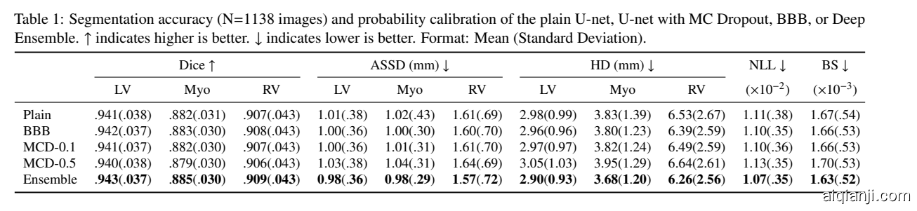
Segmentation Accuracy and Probability Calibration

The segmentation accuracy and probability calibration of the U-net trained with various methods are shown in Table segmentation_performance. Deep Ensembles performed the best in terms of segmentation accuracy and probability calibration. This was followed by BBB and MCD-0.1, which were comparable to the plain U-net. MCD-0.5 performed slightly worse than other models in terms of segmentation accuracy and probability calibration. These results indicate that Bayesian approaches or Deep Ensembles can yield similar, if not better, segmentation results compared to a plain U-net while providing uncertainty estimates at the same time.

分段精度和概率校准

具有各种方法的U-Net培训的分割精度和概率校准在表段中显示为表Semonation_Performance。在分割精度和概率校准方面，深度集合是最佳的。这是BBB和MCD-0.1，其与普通U-Net相当。根据分割精度和概率校准，MCD-0.5在其他模型中略差差。这些结果表明，贝叶斯方法或深度集合可以屈服于相似，如果不是更好的，分段结果与普通U-Net相比同时提供不确定性估计。

Uncertainty on Distorted Images

In order to validate uncertainty measures as indicators of out-of-distribution datasets, we applied the trained models to carefully generated images with various magnitudes of distortions, including: - adding Rician noise, as found in MR images , with magnitudes ranging from 0.05 to 0.10 (images intensities ranged from 0 to 1), - Gaussian blurring with a standard deviation of 1.0 to 4.0 pixels, and - deforming or stretching around the cardiac structures. Note that these distortions were not applied as part of data augmentation during training and these images were not seen by the neural network. Figure distortions_example shows examples of the distorted images. We expected decreased segmentation accuracy and increased predictive uncertainty in images with greater magnitudes of distortions.

对扭曲图像的不确定性

，以验证不确定性措施作为外部分发数据集的指标，我们应用训练型模型以仔细生成具有各种扭曲的图像，包括： - 添加瑞典噪声，如MR图像中所说，幅度范围为0.05至0.10（图像强度范围为0至1）， - 高斯模糊，标准偏差为1.0至4.0像素，围绕心脏结构变形或拉伸。请注意，这些失真未作为训练期间数据增强的一部分应用，并且神经网络未看到这些图像。 Figure Distortions_example显示扭曲图像的示例。我们预期的分割准确性降低，并提高了图像的预测性不确定性，具有更大的扭曲量大。

Trends with Increasing Distortions

Figureall_distortion_boxplots and Supplementary Table 1 show that segmentation accuracy decreased as the magnitude of the distortions (noise, gaussian blur, stretch) was increased. This is expected since these types of distortions were not seen during training and increasing the magnitude of the distortions resulted in greater differences with the original training datasets. In addition, we observed that the predictive uncertainty increased (i.e., higher predictive entropy, mutual information, ASSD, and lower Dice) with increasing magnitude of distortions but decreased after a certain threshold, as shown in Figureall_distortion_boxplots. This was the case for Deep Ensembles, BBB, and MC Dropout on images with blurring and noise distortions but not with stretching. For example, for BBB, the median predictive entropy for images with slight, moderate, and large additional noise was $ 1.66 \times 10^{-2} $ , $ 1.95 \times 10^{-2} $ , and $ 1.23 \times
10^{-2} $ , respectively. Similarly, the median ASSD for the BBB model was 0.40, 3.40, and 0.71 mm for images with slight, moderate, and large amount of blurring, respectively (See Supplementary Table 3 for more details). Figure noise_distortion_image shows examples of segmentation results and the corresponding predictive entropy and mutual information. While the increasing predictive uncertainty associated with increasing magnitude of distortions was expected, the decrease in predictive uncertainty after a threshold in cases of noise and blurring distortions was not expected. Specifically, for images that were highly distorted, all pixels were being classified as background with low uncertainty (Figureall_distortion_boxplots, bottom row). Although this seems correct when only given the labeling choice of background, LV, Myo, and RV, we argue that the distorted pixels are markedly different from the background pixels in the training images and therefore, should have high uncertainty nonetheless. This is a limitation of all the uncertainty models tested and may be improved using more expressive posteriors. Another observation is that the uncertainty measures began to fail/decrease when dramatic segmentation errors occured (Figureall_distortion_boxplots). This suggests that other heuristics or algorithms such as those presented in can be used to complement the uncertainty measures when trying to detect inaccurate segmentation. For example, segmentation with a non-circular LV blood pool or a blood volume $ < $ 50 mL is highly problematic and may indicate poor segmentation.

增加扭曲幅度后的观测

FIGURALL_DISTOL_BOXPLOT和补充表1表明，随着扭曲的幅度（噪音，高斯模糊，拉伸）增加，分割精度降低。这是预期的，因为在训练期间没有看到这些类型的扭曲，并且增加扭曲的幅度导致与原始训练数据集更大的差异。此外，我们观察到，预测性不确定性增加（即，更高的预测熵，互信息，截图和下骰子），随着较大的差异，但在某个阈值之后降低，如图所示。对于具有模糊和噪声扭曲的图像上的深度集成，BBB和MC辍学，这是如此。例如，对于BBB，具有轻微，中等和大额外噪声的图像的中值预测熵是$ 1.66 \timesT265_2{-2} $，$ 1.95 \times 1.95 {-2} $，以及$ 1.23 \times
10^\times
10^{-2} $。同样，BBB型号的中位数分别为0.40,3.40和0.71 mm，用于微小，中等和大量模糊的图像（有关更多细节，请参见补充表3）。图诊断_distorgatorrage_image显示分割结果的示例和相应的预测熵和相互信息。虽然预期噪声和模糊畸变的阈值之后的预测性不确定性增加了与增加的扭曲程度增加的预测性不确定性。具体地，对于高度扭曲的图像，所有像素都被归类为具有低不确定性的背景（FigureAll_Distorgatorration_Boxplots，底行）。虽然这似乎是正确的，但当鉴于背景，LV，MyO和RV的标签选择时，我们认为失真的像素与训练图像中的背景像素显着不同，因此，应该具有高不确定性。这是对所有测试的不确定性模型的限制，并且可以使用更多富有表现力的前后改善。另一个观察是，在发生戏剧性分割错误时，不确定性措施开始失败/减少（Figureall_distorgatorration_boxplots）。这表明，其他启发式或算法，如诸如所呈现的那些算法可以用于在试图检测到不准确的细分时补充不确定性措施。例如，具有非圆形LV血液池或血液体积$ < $ 50mL的分割非常有问题，并且可以表示分割不良。

Comparison between Deep Ensemble, BBB and MC Dropout

In terms of segmentation accuracy and probability calibration, BBB was more robust to noise distortions compared to the other methods. Specifically, BBB showed higher LV Dice, higher LV ASSD, lower NLL, and lower BS on images with greater noise distortions (Figureall_distortion_boxplots, noise = 0.07, 0.08, 0.10 and Supplementary Tables 1 and 2, degree of distortion = 2, 3, 4). Deep Ensembles was more robust to the blurring and stretching distortions than the other methods. Deep Ensembles showed higher segmentation accuracy in cases with greater blurring and stretching distortions compared to the other methods (Figureall_distortion_boxplots and Supplementary Table 1, degree of distortion = 3, 4). In terms of predictive uncertainty measures, BBB was more robust to the noise distortion while both Deep Ensembles and BBB were more resistant to the blurring compared to the other methods. For example, the mutual information, Dice, and ASSD uncertainty measures peaked at a noise distortion with degree=3 for BBB. In contrast, the uncertainty measures peaked at a noise distortion with degree=2 for Deep Ensemble, MCD-0.1, and MCD-0.5. Comparing the uncertainty on images with heavy noise distortions (degree of distortion = 3, 4), BBB showed the highest predictive uncertainty. This was followed by MCD-0.5 while Deep Ensembles and MCD-0.1 showed the lowest predictive uncertainties. For images that were heavily blurred, Deep Ensembles and BBB showed the highest predictive uncertainty. In cases of images with stretching distortions, all methods showed fairly similar predictive uncertainty across all degrees of stretching. Having high predictive uncertainties on heavily distorted images is desirable since they have lower segmentation accuracy. Overall, BBB showed good predictive uncertainties on all of the tested distortions while Deep Ensemble showed good predictive uncertainties only in cases of blurring and stretching distortions. MCD-0.1 and MCD-0.5 showed results comparable to BBB and Deep Ensembles only on the stretched datasets.

Deep Ensemble, BBB and MC Dropout的比较

之间的比较，与其他方法相比，BBB对噪声扭曲更加坚固。具体地，BBB在具有更大噪声失真的图像上显示出更高的LV骰子，更高的LV ASSD，更低的NLL和下BS（Figureall_Distorgatory_BoxPlots，噪声= 0.07,0.08,0.07，0.08,0.10和补充表1和2，失真程度= 2,3,4 ）。深度集合对模糊和拉伸扭曲比其他方法更加强大。与其他方法相比，在更大的模糊和拉伸扭曲的情况下，深度集成精度在更大的模糊和拉伸扭曲（Figurealll_distorgatory_boxpots和补充表1的情况下，失真= 3,4）。就预测性不确定性措施而言，与其他方法相比，BBB对噪声失真更加强劲地对噪声失真更耐受模糊更耐受模糊。例如，相互信息，骰子和ASSD不确定性测量以BBB的度= 3的噪声失真达到峰值。相反，不确定度测量以深度= 2的噪声失真达到峰值，用于深集合，MCD-0.1和MCD-0.5。比较具有重度噪声扭曲的图像的不确定性（畸变程度= 3,4），BBB显示出最高的预测性不确定性。接下来是MCD-0.5，而深度集成和MCD-0.1显示出最低的预测性不确定性。对于严重模糊的图像，深度合奏和BBB显示出最高的预测性不确定性。在具有拉伸扭曲的图像的情况下，所有方法在所有伸展程度上都显示出相同的预测性不确定性。由于它们具有较低的分割精度，因此希望具有高预测性的不确定性。总体而言，BBB对所有测试扭曲显示出良好的预测性不确定因素，而深度集合仅在模糊和拉伸扭曲的情况下显示出良好的预测性不确定性。 MCD-0.1和MCD-0.5显示出与BBB和深度仅在拉伸的数据集上相当的结果。

Uncertainty on Dataset Shift

To further validate the uncertainty measures, we applied the models trained on the UKBB dataset to a different dataset - the ACDC dataset. The ACDC dataset consists of images with pathologies and image contrast distinctly different from the UKBB training dataset. Because of the dataset shift, we expect decreased segmentation accuracy and increased predictive uncertainty on the ACDC dataset compared to the UKBB test dataset. Figure metrics_correlations shows the segmentation accu

[论文翻译]Estimating Uncertainty in Neural Networks for Cardiac MRI Segmentation: A Benchmark Study

原文地址：https://arxiv.org/pdf/2012.15772v1.pdf