4D Attention-based Neural Network for EEG Emotion Recognition
基于4D注意力机制的神经网络在EEG情绪识别中的应用
Abstract
摘要
Electroencephalograph (EEG) emotion recognition is a significant task in the brain-computer interface field. Although many deep learning methods are proposed recently, it is still challenging to make full use of the information contained in different domains of EEG signals. In this paper, we present a novel method, called four-dimensional attention-based neural network (4D-aNN) for EEG emotion recognition. First, raw EEG signals are transformed into 4D spatial-spectral-temporal representations. Then, the proposed 4D-aNN adopts spectral and spatial attention mechanisms to adaptively assign the weights of different brain regions and frequency bands, and a convolutional neural network (CNN) is utilized to deal with the spectral and spatial information of the 4D representations. Moreover, a temporal attention mechanism is integrated into a bidirectional Long Short-Term Memory (LSTM) to explore temporal dependencies of the 4D representations. Our model achieves state-of-the-art performance on the SEED dataset under intra-subject splitting. The experimental results have shown the effectiveness of the attention mechanisms in different domains for EEG emotion recognition.
脑电图(EEG)情绪识别是脑机接口领域的重要任务。尽管近期提出了许多深度学习方法,但如何充分利用EEG信号不同域的信息仍具挑战性。本文提出了一种基于四维注意力神经网络(4D-aNN)的新方法:首先将原始EEG信号转换为4D空间-频谱-时间表征;随后4D-aNN采用频谱和空间注意力机制自适应分配不同脑区与频段的权重,并利用卷积神经网络(CNN)处理4D表征的频谱和空间信息;此外,通过将时间注意力机制整合到双向长短期记忆网络(LSTM)中,探索4D表征的时间依赖性。我们的模型在SEED数据集上实现了被试内划分的最优性能,实验结果证明了不同域注意力机制对EEG情绪识别的有效性。
Keywords: EEG, emotion recognition, attention mechanism, convolutional recurrent neural network
关键词:EEG、情绪识别、注意力机制、卷积循环神经网络
Introduction
引言
Emotion plays an important role in daily life and is closely related to human behavior and cognition (Dolan 2002). As one of the most significant research topics of affective computing, emotion recognition has received increasing attention in recent years for its applications of disease detection (Bamdad et al. 2015; Figueiredo et al. 2019), human-computer interaction (Fiorinia et al. 2020; Kat si gianni s and Ramzan 2017), and workload estimation (Blankertz et al. 2016). In general, emotion recognition methods can be divided into two categories (Mühl et al. 2014). One is based on external emotion responses including facial expressions and gestures(Yan et al. 2016), and the other is based on internal emotion responses including electroencephalograph (EEG) and electrocardiograph y (ECG) (Zheng et al. 2017). Neuro scientific researches have shown that some major brain cortex regions are closely related to emotions, making it possible to decode emotions based on EEG (Brittona et al. 2006; Lotfia and Akbarzadeh-T 2014). EEG is non-invasive, portable, and inexpensive so that it has been widely used in the field of brain-computer interfaces (BCIs) (P furt sc heller et al. 2010). Besides, EEG signals contain various spatial, spectral, and temporal information about emotions evoked by specific stimulation patterns. Therefore, more and more researchers concentrate on EEG emotion recognition recently (Alhagry et al. 2017; Li and Lu 2009).
情绪在日常生活中扮演着重要角色,并与人类行为及认知密切相关 (Dolan 2002)。作为情感计算最重要的研究课题之一,情绪识别因其在疾病检测 (Bamdad et al. 2015; Figueiredo et al. 2019)、人机交互 (Fiorini et al. 2020; Katsigiannis and Ramzan 2017) 和工作负荷评估 (Blankertz et al. 2016) 等领域的应用价值,近年来受到越来越多的关注。一般而言,情绪识别方法可分为两类 (Mühl et al. 2014):一类基于外部情绪反应(如面部表情和手势)(Yan et al. 2016),另一类则基于内部情绪反应(如脑电图 (EEG) 和心电图 (ECG))(Zheng et al. 2017)。神经科学研究表明,某些主要大脑皮层区域与情绪密切相关,这使得基于 EEG 解码情绪成为可能 (Britton et al. 2006; Lotfi and Akbarzadeh-T 2014)。EEG 具有非侵入性、便携且成本低廉的特点,因此在脑机接口 (BCI) 领域得到广泛应用 (Pfurtscheller et al. 2010)。此外,EEG 信号包含了由特定刺激模式诱发情绪的各种空间、频谱和时域信息。因此,近年来越来越多的研究者专注于 EEG 情绪识别研究 (Alhagry et al. 2017; Li and Lu 2009)。
Traditional EEG emotion recognition methods usually extract hand-crafted features from EEG signals first and then adopt shallow models to classify the emotion features. EEG emotion features can be extracted from the time domain, frequency domain, and time-frequency domain. Jenke et al. conduct a comprehensive survey on EEG feature extraction methods by using machine learning techniques on a selfrecorded dataset (Jenke et al. 2014). For classifying the extracted emotion features, many researchers have adopted machine learning methods over the past few years (Kim et al. 2013). Li et al. apply a linear support vector machine (SVM) to classify emotion features extracted from the gamma frequency band (Li and Lu 2009). Duan et al. extract differential entropy (DE) features, which are superior to representing emotion states in EEG signals (Shi et al. 2013), from multichannel EEG data and combine a $\mathrm{k\Omega}$ -Nearest Neighbor (KNN) with SVM to classify the DE features (Duan et al. 2013). However, shallow models require lots of expert knowledge to design and select emotion features, limiting their performance on EEG emotion classification.
传统的脑电图(EEG)情绪识别方法通常先从EEG信号中提取手工特征,再采用浅层模型对情绪特征进行分类。EEG情绪特征可从时域、频域和时频域中提取。Jenke等人在自录数据集上使用机器学习技术对EEG特征提取方法进行了全面调研(Jenke et al. 2014)。对于已提取情绪特征的分类,过去几年许多研究者采用了机器学习方法(Kim et al. 2013)。Li等人应用线性支持向量机(SVM)对从gamma频段提取的情绪特征进行分类(Li and Lu 2009)。Duan等人从多通道EEG数据中提取差分熵(DE)特征(Shi et al. 2013),并将k近邻(KNN)与SVM结合对DE特征进行分类(Duan et al. 2013)。然而,浅层模型需要大量专家知识来设计和选择情绪特征,这限制了其在EEG情绪分类上的性能。
Deep learning methods have been demonstrated to outperform traditional machine learning methods in many fields such as computer vision, natural language processing, and biomedical signal processing (Abbass et al. 2018; Craik et al. 2019) for the ability to learn high-level features from data automatically (Krizhevsky et al. 2012). Recently, some researchers have applied deep learning to EEG emotion recognition. Zheng et al. introduce a deep belief network (DBN) to investigate the critical frequency bands and EEG signal channels for EEG emotion recognition (Zheng and Lu 2015). Yang et al. propose a hierarchical network to classify the DE features extracted from different frequency bands (Yang et al. 2018b). Song et al. use a graph convolutional neural network to classify the DE features (Song et al. 2020). Ma et al. propose a multimodal residual Long Short-Term Memory model (MMResLSTM) for emotion recognition, which shares temporal weights across the multiple modalities (Jiaxin Ma et al. 2019). To learn the bi-hemispheric discrepancy for EEG emotion recognition, Yang et al. propose a novel bi-hemispheric discrepancy model (BiHDM) (Li et al. 2020). All those deep learning methods outperform the shallow models.
深度学习方法在计算机视觉、自然语言处理和生物医学信号处理等多个领域已被证明优于传统机器学习方法 (Abbass et al. 2018; Craik et al. 2019),因其具备从数据中自动学习高级特征的能力 (Krizhevsky et al. 2012)。近年来,一些研究者将深度学习应用于脑电(EEG)情绪识别。Zheng等采用深度信念网络(DBN)探究脑电情绪识别中的关键频段与信号通道 (Zheng and Lu 2015)。Yang等提出分层网络对从不同频段提取的微分熵(DE)特征进行分类 (Yang et al. 2018b)。Song等使用图卷积神经网络对微分熵特征进行分类 (Song et al. 2020)。Ma等提出多模态残差长短时记忆模型(MMResLSTM)进行情绪识别,该模型在多个模态间共享时序权重 (Jiaxin Ma et al. 2019)。为学习脑电情绪识别的双半球差异特征,Yang等提出新型双半球差异模型(BiHDM) (Li et al. 2020)。这些深度学习方法均优于浅层模型。
Although deep learning emotion recognition models have achieved higher accuracy than shallow models, it is still challenging to fuse more important information on different domains and capture disc rim i native local patterns in EEG signals. In the past decades, many researchers have investigated the critical frequency bands and channels for EEG emotion recognition. Zheng et al. demonstrate that $\mathsf{\beta}[14{\sim}31\mathrm{Hz}]$ and $\gamma[31{\sim}51~\mathrm{Hz}]$ bands are more related to emotion recognition than other bands, and their model achieves the best performance when combining all frequency bands. They also conduct experiments to select critical channels and propose the minimum pools of electrode sets for emotion recognition (Zheng and $\mathrm{Lu}2015\$ . To utilize the spatial information of EEG signals, Li et al. propose a 2D sparse map to maintain the information hidden in the electrode placement (Li et al. 2018). Zhong et al. introduce a regularized graph neural network (RGNN) to capture both local and global relations among different EEG channels for emotion recognition (Zhong et al. 2020). The temporal dependencies in EEG signals are also important to emotion recognition. For example, Ma et al. (Jiaxin Ma et al. 2019) apply LSTMs in their models to extract temporal features for emotion recognition. Shen et al. transform the DE features of different channels into 4D structures to integrate the spectral, spatial, and temporal information simultaneously and then use a fourdimensional convolutional recurrent neural network (4DCRNN) to recognize different emotions (Shen et al. 2020). However, the differences among brain regions and frequency bands are not fully utilized in their work. To adaptively capture disc rim i native patterns in EEG signals, attention mechanisms have been applied to EEG emotion recognition. For instance, Tao et al. introduce a channel-wise attention mechanism, assigning the weights of different channels adaptively, along with an extended self-attention to explore the temporal dependencies of EEG signals (Tao et al. 2020). Jia et al. propose a two-stream network with attention mechanisms to adaptively focus on important patterns (Jia et al. 2020). From the above, it can be observed that it is critical to integrate information on different domains and adaptively capture important brain regions, frequency bands, and timestamps in a unified network for EEG emotion recognition.
虽然深度学习情感识别模型相比浅层模型取得了更高的准确率,但在融合多领域重要信息以及捕捉脑电信号中的判别性局部模式方面仍存在挑战。过去几十年间,许多研究者探索了脑电情感识别中的关键频段与通道。Zheng等人证明β[14 31 Hz]和γ[31~51 Hz]频段比其他频段与情感识别更具相关性,其模型在融合所有频段时达到最佳性能。他们还通过实验筛选关键通道,提出了情感识别所需的最小电极集组合(Zheng and Lu 2015)。为利用脑电信号的空间信息,Li等人提出二维稀疏映射来保持电极排布中隐含的信息(Li et al. 2018)。Zhong等人采用正则化图神经网络(RGNN)来捕捉不同脑电通道间的局部与全局关系(Zhong et al. 2020)。脑电信号的时序依赖性对情感识别同样重要,例如Ma等人在模型中运用LSTM提取时序特征(Jiaxin Ma et al. 2019)。Shen等人将不同通道的微分熵特征转换为4D结构以同步整合频谱、空间和时序信息,再通过四维卷积循环神经网络(4D-CRNN)进行情感识别(Shen et al. 2020),但其工作未充分利用脑区与频段间的差异性。为自适应捕捉脑电信号中的判别模式,注意力机制已被应用于该领域:Tao等人提出通道注意力机制自适应分配通道权重,并扩展自注意力来探索信号时序依赖性(Tao et al. 2020);Jia等人开发了具有注意力机制的双流网络来自适应聚焦重要模式(Jia et al. 2020)。由此可见,构建统一网络来整合多领域信息并自适应捕捉关键脑区、频段及时间点,对脑电情感识别至关重要。
In this paper, we propose a four-dimensional attentionbased neural network named 4D-aNN for EEG emotion recognition. First, we transform raw EEG signals into 4D spatial-spectral-temporal representations which consist of several temporal slices. Different brain regions and frequency bands vary in the contributions to EEG emotion recognition, and the temporal dependencies of 4D representations should also be considered. Therefore, we employ attention mechanisms on both a CNN and a bidirectional LSTM network to adaptively capture disc rim i native patterns. For the CNN model, the attention mechanism is applied to the spatial and spectral dimensions of each temporal slice so that the important brain regions and frequency bands could be captured. As for the bidirectional LSTM model, the attention mechanism is applied to utilize long-range temporal dependencies so that the importance of different temporal slices in one 4D representation could be fully explored.
本文提出了一种基于四维注意力机制的神经网络4D-aNN,用于脑电图(EEG)情绪识别。首先,我们将原始EEG信号转换为由多个时间切片组成的四维空间-频谱-时间表征。不同脑区和频段对EEG情绪识别的贡献度存在差异,同时还需考虑四维表征的时间依赖性。为此,我们在CNN和双向LSTM网络中均采用了注意力机制来自适应捕捉判别性特征。对于CNN模型,注意力机制作用于每个时间切片的空间和频谱维度,以捕获重要的脑区与频段信息;而在双向LSTM模型中,注意力机制用于利用长程时间依赖性,从而充分挖掘单个四维表征中不同时间切片的重要性。
The primary contribution of this paper are summarized as follows: a) We propose a four-dimensional attention-based neural network, which fuses information on different domains and captures disc rim i native patterns in EEG signals based on the 4D spatial-spectral-temporal representation. b) We conduct experiments on the SEED dataset, and the experimental results indicate that our model achieves state-ofthe-art performance under intra-subject splitting.
本文的主要贡献总结如下:
a) 我们提出了一种基于四维注意力机制的神经网络,该网络融合了不同领域的信息,并基于4D空间-频谱-时间表征捕捉了EEG信号中的判别性模式。
b) 我们在SEED数据集上进行了实验,结果表明,在受试者内划分条件下,我们的模型实现了最先进的性能。
The remainder of this paper is organized as follows. We describe our proposed method in the Method section. Dataset, experiment settings, results, ablation studies, and discussion are presented in the Experiment section. Finally, conclusions are given in the Conclusion section.
本文的其余部分组织如下。方法部分介绍了我们提出的方法。实验部分展示了数据集、实验设置、结果、消融研究和讨论。最后,结论部分给出了总结。
Method
方法
Figure 1 illustrates the overall structure of 4D-aNN for EEG emotion recognition. It consists of the 4D spatial-spectraltemporal representation, the attention-based CNN, the attention-based bidirectional LSTM, and the classifier. We will describe the details of each part in sequence.
图 1: 展示了用于脑电图 (EEG) 情绪识别的4D-aNN整体结构。该结构包含4D空间-频谱-时间表征、基于注意力的CNN、基于注意力的双向LSTM以及分类器。我们将依次描述每个部分的细节。
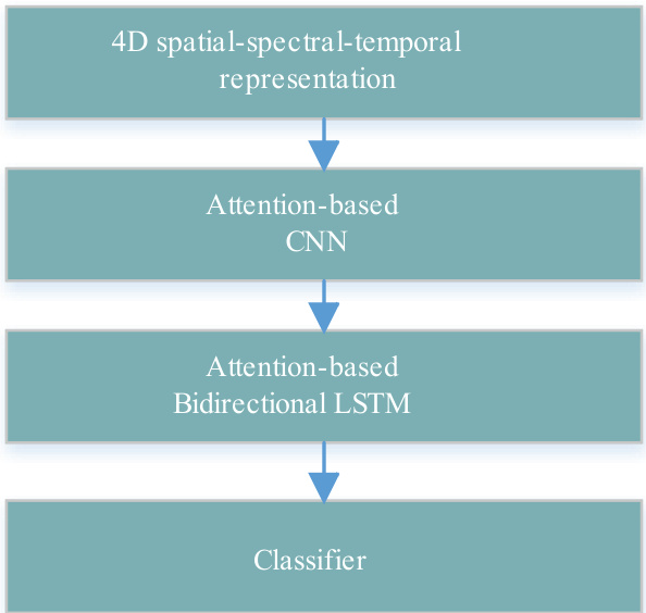
Fig. 1 The overall structure of 4D-aNN.
图 1: 4D-aNN的整体结构。
4D spatial-spectral-temporal representation
4D 空间-光谱-时间表示
The process of generating 4D representation is depicted in Fig. 2. As previous works do (Shen et al. 2020; Yang et al. 2018a), we split original EEG signals into $T$ seconds long segments without overlapping. Each segment is assigned with the same label as the original EEG signals. Then we decompose each segment into five frequency bands (i.e. δ[1~4 Hz], $\mathsf{\theta}[4{\sim}8\mathrm{Hz}]$ , $\mathsf{a}[8{\sim}14~\mathrm{HZ}]$ , $3[14{\sim}31~\mathrm{Hz}]$ , and $\gamma[31{\sim}51~\mathrm{Hz}].$ ) with five-order Butterworth filters. The Differential Entropy (DE) features and Power Spectral Density (PSD) features of all EEG channels, which have been proven to be effective for emotion recognition (Zheng et al. 2017), are extracted from five frequency bands respectively with a 0.5s window for each segment.
图 2: 展示了4D表征的生成过程。如先前工作(Shen et al. 2020; Yang et al. 2018a)所述,我们将原始EEG信号分割为$T$秒长的无重叠片段,每个片段保留原始EEG信号的标签。随后使用五阶巴特沃斯滤波器将每个片段分解为五个频带(即δ[1 4 Hz]、$\mathsf{\theta}[4{\sim}8\mathrm{Hz}]$、$\mathsf{a}[8{\sim}14~\mathrm{HZ}]$、$3[14{\sim}31~\mathrm{Hz}]$和$\gamma[31{\sim}51~\mathrm{Hz}]$)。从每个片段的0.5秒窗口中,分别提取所有EEG通道的微分熵(Differential Entropy, DE)特征和功率谱密度(Power Spectral Density, PSD)特征,这些特征已被证明对情绪识别有效(Zheng et al. 2017)。
PSD is defined as
PSD 定义为
$$
h_{P}(X)=E[x^{2}]
$$
$$
h_{P}(X)=E[x^{2}]
$$
where $x$ is formally a random variable and in this context, the signal acquired from a certain frequency band on a certain EEG channel.
其中 $x$ 在形式上是一个随机变量,在此上下文中表示从某个EEG通道的特定频带采集到的信号。
DE feature is capable of discriminating EEG patterns between low and high frequency energy, which is defined as
DE特征能够区分低频与高频能量之间的脑电图模式
$$
h_{D}(X)=-\int_{X}f(x)\log{\big(}f(x){\big)}d x
$$
$$
h_{D}(X)=-\int_{X}f(x)\log{\big(}f(x){\big)}d x
$$
where $f(x)$ is the probability density function of $x$ . If $x$ obeys the Gaussian distribution $N(\mu,\sigma^{2})$ , DE can simply be calculated by the following formulation:
其中 $f(x)$ 是 $x$ 的概率密度函数。若 $x$ 服从高斯分布 $N(\mu,\sigma^{2})$,则DE可通过以下公式简单计算:
$$
\begin{array}{c}{{h_{D}(X)=\displaystyle-\int_{-\infty}^{\infty}\frac{1}{\sqrt{2\pi\sigma^{2}}}e x p\frac{(x-\mu)^{2}}{2\sigma^{2}}\log\frac{1}{\sqrt{2\pi\sigma^{2}}}e x p\frac{(x-\mu)^{2}}{2\sigma^{2}}d x}}\ {{=\displaystyle\frac{1}{2}\log2\pi e\sigma^{2}(3)~}}\end{array}
$$
$$
\begin{array}{c}{{h_{D}(X)=\displaystyle-\int_{-\infty}^{\infty}\frac{1}{\sqrt{2\pi\sigma^{2}}}e x p\frac{(x-\mu)^{2}}{2\sigma^{2}}\log\frac{1}{\sqrt{2\pi\sigma^{2}}}e x p\frac{(x-\mu)^{2}}{2\sigma^{2}}d x}}\ {{=\displaystyle\frac{1}{2}\log2\pi e\sigma^{2}(3)~}}\end{array}
$$
where $e$ and $\sigma$ are Euler’s constant and standard deviation of $x$ , respectively.
其中 $e$ 和 $\sigma$ 分别为欧拉常数和 $x$ 的标准差。
Thus, We extract a 3D feature tensor $F_{n}\in R^{c x2f x2T},n=$ $1,2,\ldots,N$ from each segment, where $N$ is the number of total segments, $c$ is the number of EEG channels, $2f$ represents DE and PSD features of $f$ frequency bands, and $2T$ is derived by the 0.5s window without overlapping. To utilize the spatial information of electrodes, we organize all the $c$ channels as a 2D sparse map so that the 3D feature tensor $F_{n}$ is transformed into a 4D representation $X_{n}\in R^{h\times w\times2f\times2T}$ , where $h$ and $w$ are the height and width of the 2D sparse map, respectively. The 2D sparse map of all the c channels with zero-padding is shown in Fig. 3, which preserves the topology of different electrodes. In this paper, we set $h=19$ , $w=19$ , and $f=5$ .
因此,我们从每个片段中提取一个3D特征张量 $F_{n}\in R^{c x2f x2T},n=$ $1,2,\ldots,N$ ,其中 $N$ 是总片段数, $c$ 是EEG通道数, $2f$ 表示 $f$ 个频段的DE和PSD特征, $2T$ 由无重叠的0.5秒窗口生成。为了利用电极的空间信息,我们将所有 $c$ 个通道组织成一个2D稀疏映射,从而将3D特征张量 $F_{n}$ 转换为4D表示 $X_{n}\in R^{h\times w\times2f\times2T}$ ,其中 $h$ 和 $w$ 分别是2D稀疏映射的高度和宽度。图3展示了所有c通道的零填充2D稀疏映射,该映射保留了不同电极的拓扑结构。本文中,我们设置 $h=19$ , $w=19$ ,以及 $f=5$ 。
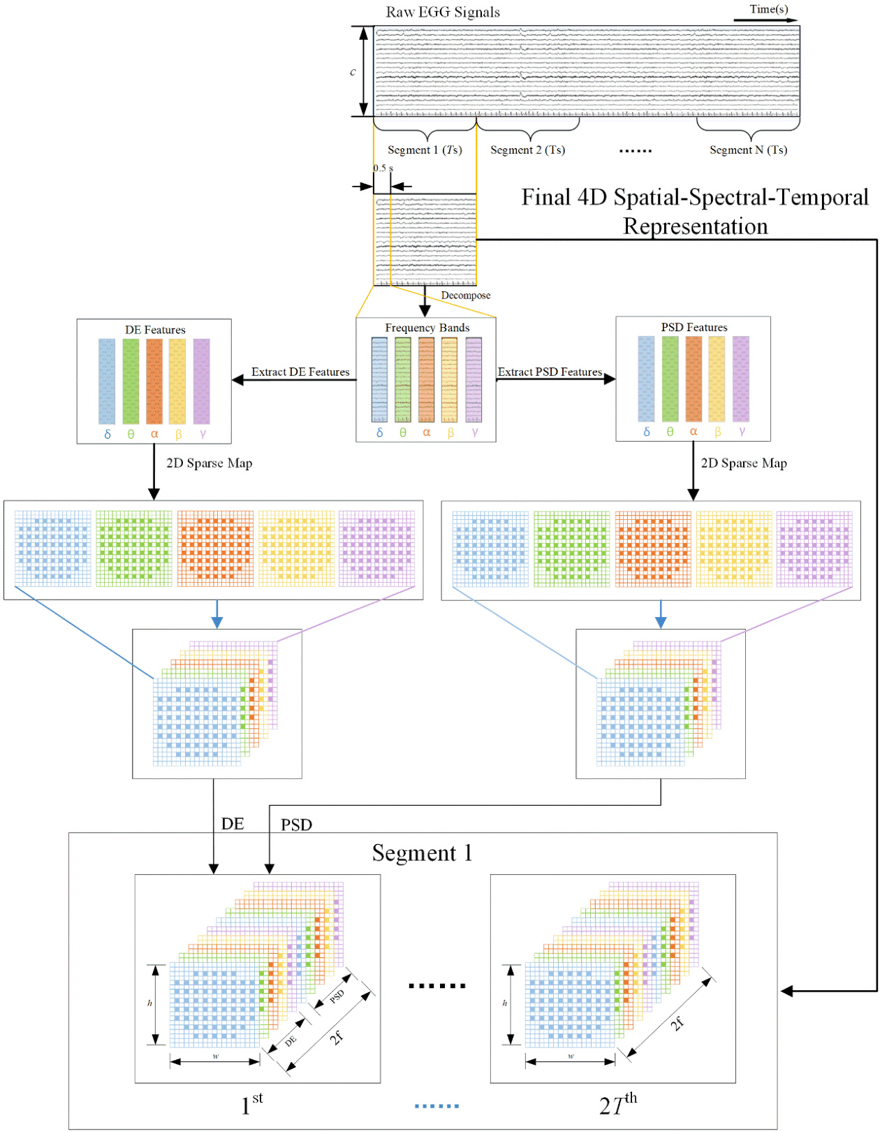
Fig. 2 The generation of 4D spatial-spectral-temporal representation. For each Ts EEG signal segment, we extract DE and PSD features from different channels and frequency bands with a 0.5s window. Then, the features are transformed into a 4D representation which consists of 2T temporal slices.
图 2: 4D空间-频谱-时间表征的生成过程。对于每个Ts时长的EEG信号片段,我们使用0.5秒窗口从不同通道和频段提取DE(微分熵)和PSD(功率谱密度)特征。随后,这些特征被转换为包含2T个时间切片的4D表征。
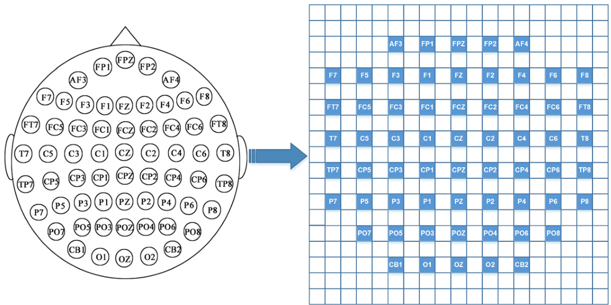
Fig. 3 The 2D sparse map with zero-padding of 62 channels. The purpose of the organization is to preserve the positional relationships among different electrodes.
图 3: 采用62通道零填充的二维稀疏映射图。该布局旨在保持不同电极之间的位置关系。
Attention-based CNN
基于注意力的CNN
For a 4D spatial-spectral-temporal representation $X_{n}$ , we extract the spatial and spectral information from each temporal slice $S_{i}\in R^{h\times w\times2f},i~=~1,2,\ldots,2T$ with a CNN, explore the disc rim i native local patterns in spatial and spectral domains with a convolutional attention module, and finally get its spatial and spectral representation. The attention module here is similar to what Woo et al. propose (Woo et al. 2018), which is originally used to improve the representation power of CNN networks.
对于一个4D空间-光谱-时间表征 $X_{n}$,我们从每个时间切片 $S_{i}\in R^{h\times w\times2f},i~=~1,2,\ldots,2T$ 中通过CNN提取空间和光谱信息,利用卷积注意力模块探索空间和光谱域中的判别性局部模式,最终获得其空间和光谱表征。这里的注意力模块类似于Woo等人提出的方法 (Woo et al. 2018),最初用于提升CNN网络的表征能力。
The structure of the attention-based CNN is shown in Fig. 4. It contains four convolutional layers, four convolutional attention modules, one max-pooling layer, and one fullyconnected layer. The four convolutional layers have 64, 128, 256, and 64 feature maps with the filter size of $5\times5$ , $5\times5$ , $5\times5$ , and $3\times3$ , respectively. Specifically, a convolutional attention module is used after each convolutional layer to utilize the spatial and spectral attention mechanisms, and the details will be given later. We only use one max-pooling layer with a filter size of $2\times2$ after the last convolutional attention module to preserve more information and enhance the robustness of the network. Finally, outputs of the max-pooling layer are flattened and fed to the fully-connected layer with 150 units. Thus, for each temporal slice $S_{i}$ , we take the final output $P_{i}\in R^{150}$ as its spatial and spectral representation.
基于注意力机制的 CNN 结构如图 4 所示。它包含四个卷积层、四个卷积注意力模块、一个最大池化层和一个全连接层。四个卷积层分别具有 64、128、256 和 64 个特征图,滤波器大小分别为 $5\times5$ 、 $5\times5$ 、 $5\times5$ 和 $3\times3$ 。具体而言,每个卷积层后都使用一个卷积注意力模块来利用空间和光谱注意力机制,细节将在后文给出。我们仅在最后一个卷积注意力模块后使用一个滤波器大小为 $2\times2$ 的最大池化层,以保留更多信息并增强网络的鲁棒性。最后,将最大池化层的输出展平并输入具有 150 个单元的全连接层。因此,对于每个时间切片 $S_{i}$ ,我们将最终输出 $P_{i}\in R^{150}$ 作为其空间和光谱表示。
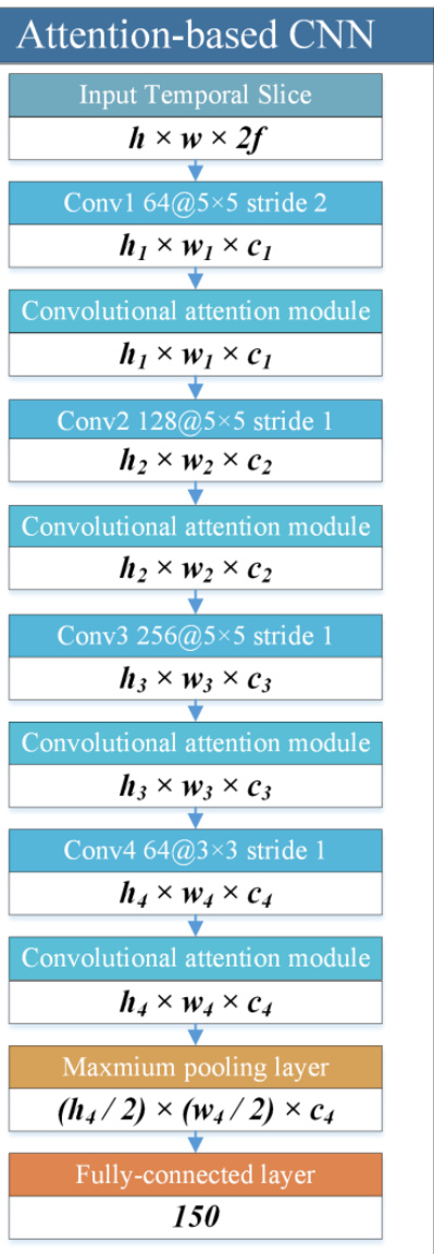
Fig. 4 The structure of the attention-based CNN. The upper half of the blocks in the figure is the type of layers and the lower denotes the shape of its output tensors.
图 4: 基于注意力机制的 CNN (Convolutional Neural Network) 结构。图中模块上半部分表示层类型,下半部分表示其输出张量的形状。
Convolutional attention module
卷积注意力模块
The convolutional attention module is applied after each convolutional layer to adaptively capture important brain regions and frequency bands. The structure of the convolutional attention module is shown in Fig. 5. It consists of two sub-modules, i.e. the spatial attention module and the spectral attention module.
卷积注意力模块被应用于每个卷积层之后,以自适应地捕捉重要脑区和频段。卷积注意力模块的结构如图5所示,由两个子模块组成,即空间注意力模块和频谱注意力模块。
For each convolutional layer above, its output is a 3D feature tensor $V\in R^{h_{v}\times w_{v}\times c_{v}}$ , where $h_{v}$ , $w_{v}$ , and $c_{v}$ are the height of the 2D feature maps of $V$ , the width of the 2D feature maps of $V$ , and the number of the 2D feature maps of $V$ , respectively. We take $V$ as the input of the convolutional attention module.
对于上述每个卷积层,其输出是一个3D特征张量 $V\in R^{h_{v}\times w_{v}\times c_{v}}$ ,其中 $h_{v}$ 、 $w_{v}$ 和 $c_{v}$ 分别表示 $V$ 的2D特征图高度、宽度以及特征图数量。我们将 $V$ 作为卷积注意力模块的输入。
The spectral attention module is applied to identify valuable frequency bands for emotion recognition. The average pooling has been widely used to aggregate spatial information and the maximum pooling has been commonly adopted to gather distinctive features. Therefore, we shrink the spatial dimension of $V$ by a spatial-wise average pooling and a spatial-wise maximum pooling, which are defined as:
谱注意力模块用于识别情感识别中有价值的频段。平均池化 (average pooling) 被广泛用于聚合空间信息,而最大池化 (maximum pooling) 则常用于收集显著特征。因此,我们通过空间维度的平均池化和最大池化来缩小 $V$ 的空间维度,其定义如下:
$$
\begin{array}{l}{{\displaystyle{\cal C}{a v g,i}=\frac{1}{h_{v}\times w_{v}}\sum_{h=1}^{h_{v}}\sum_{w=1}^{\bar{w}{v}}V_{i}\left(h,w\right),i=1,2,\ldots,c_{v}}}\ {{\displaystyle{\cal C}{m a x,i}=m a x(V_{i}),i=1,2,\ldots,c_{v}}}\end{array}
$$
$$
\begin{array}{l}{{\displaystyle{\cal C}{a v g,i}=\frac{1}{h_{v}\times w_{v}}\sum_{h=1}^{h_{v}}\sum_{w=1}^{\bar{w}{v}}V_{i}\left(h,w\right),i=1,2,\ldots,c_{v}}}\ {{\displaystyle{\cal C}{m a x,i}=m a x(V_{i}),i=1,2,\ldots,c_{v}}}\end{array}
$$
where $V_{i}\in R^{h_{v}\times w_{v}}$ denotes the 2D feature map in the $i{-}t h$ channel of $V$ , $C_{a v g,i}$ represents the element in the i-th channel of the spatial average representation $C_{a v g}\in R^{c_{v}}$ , $m a x(Z)$ returns the largest element in $Z$ , and $C_{m a x,i}$ is the element in the $i{-}t h$ channel of the spatial maximum representation $C_{m a x}\in R^{c_{v}}$ . Subsequently, we implement the spectral attention by two fully-connected layers, a Relu activation function and a sigmoid activation function, which is defined as:
其中 $V_{i}\in R^{h_{v}\times w_{v}}$ 表示 $V$ 的第 $i{-}t h$ 通道的二维特征图,$C_{a v g,i}$ 代表空间平均表示 $C_{a v g}\in R^{c_{v}}$ 中第i个通道的元素,$m a x(Z)$ 返回 $Z$ 中的最大元素,$C_{m a x,i}$ 是空间最大表示 $C_{m a x}\in R^{c_{v}}$ 的第 $i{-}t h$ 通道元素。随后,我们通过两个全连接层、一个Relu激活函数和一个sigmoid激活函数来实现频谱注意力机制,其定义为:
$$
\begin{array}{r l}{{}}&{{\displaystyle A_{s p e c t r a l,a v g}=W_{2}^{S}(R e l u(W_{1}^{S}C_{a v g})}}\ {{}}&{{\displaystyle A_{s p e c t r a l,m a x}=W_{2}^{S}(R e l u(W_{1}^{S}C_{m a x})}}\ {{}}&{{\displaystyle A_{s p e c t r a l}=s i g m o i d\big(A_{s p e c t r a l,a v g}\oplus A_{s p e c t r a l,m a x}\big)}}\ {{}}&{{\displaystyle R e l u(x)=\operatorname*{max}(x,0)}}\ {{}}&{{\displaystyle s i g m o i d(x)=\frac{1}{1+~e^{-x}}}}\end{array}
$$
$$
\begin{array}{r l}{{}}&{{\displaystyle A_{s p e c t r a l,a v g}=W_{2}^{S}(R e l u(W_{1}^{S}C_{a v g})}}\ {{}}&{{\displaystyle A_{s p e c t r a l,m a x}=W_{2}^{S}(R e l u(W_{1}^{S}C_{m a x})}}\ {{}}&{{\displaystyle A_{s p e c t r a l}=s i g m o i d\big(A_{s p e c t r a l,a v g}\oplus A_{s p e c t r a l,m a x}\big)}}\ {{}}&{{\displaystyle R e l u(x)=\operatorname*{max}(x,0)}}\ {{}}&{{\displaystyle s i g m o i d(x)=\frac{1}{1+~e^{-x}}}}\end{array}
$$
where $W_{1}^{S}$ and $W_{2}^{S}$ are learnable parameters, $\textcircled{4}$ denotes the element-wise addition, and $A_{s p e c t r a l}\in R^{1\times1\times c_{v}}$ is the spectral attention. The elements of $A_{s p e c t r a l}$ represent the importance of the corresponding 2D feature maps of the spectral domain. After generating the spectral attention $A_{s p e c t r a l}$ , the output of the spectral attention module can be defined as:
其中 $W_{1}^{S}$ 和 $W_{2}^{S}$ 是可学习参数,$\textcircled{4}$ 表示逐元素相加,$A_{s p e c t r a l}\in R^{1\times1\times c_{v}}$ 是光谱注意力。$A_{s p e c t r a l}$ 的元素代表光谱域对应二维特征图的重要性。生成光谱注意力 $A_{s p e c t r a l}$ 后,光谱注意力模块的输出可定义为:
$$
V^{\prime}=A_{s p e c t r a l}\otimes V
$$
$$
V^{\prime}=A_{s p e c t r a l}\otimes V
$$
where $V^{\prime}$ denotes the refined 3D feature tensor, and $\otimes$ represents the element-wise multiplication.
其中 $V^{\prime}$ 表示精炼后的3D特征张量,$\otimes$ 代表逐元素相乘。
The spatial attention module is applied to identify valuable brain regions for emotion recognition. Firstly, we shrink the spectral dimension of $V^{\prime}$ by spectral-wise average pooling and spectral-wise maximum pooling, which is defined as:
空间注意力模块用于识别对情绪识别有价值的脑区。首先,我们通过谱维平均池化和谱维最大池化缩减 $V^{\prime}$ 的频谱维度,其定义为:
$$
\begin{array}{c l}{{}}&{{S p h_{a v g,(h,w)}=\displaystyle\frac{1}{c_{v}}\sum_{c=1}^{c_{v}}S_{h,w}^{\prime}(c),h=1,2,\ldots,h_{v};w}}\ {{}}&{{=\displaystyle1,2,\ldots,w_{v}}}\ {{}}&{{S P A_{m a x,(h,w)}=\displaystyle m a x(S_{h,w}^{\prime}),h=1,2,\ldots,h_{v};w}}\ {{}}&{{=\displaystyle1,2,\ldots,w_{v}}}\end{array}
$$
$$
\begin{array}{c l}{{}}&{{S p h_{a v g,(h,w)}=\displaystyle\frac{1}{c_{v}}\sum_{c=1}^{c_{v}}S_{h,w}^{\prime}(c),h=1,2,\ldots,h_{v};w}}\ {{}}&{{=\displaystyle1,2,\ldots,w_{v}}}\ {{}}&{{S P A_{m a x,(h,w)}=\displaystyle m a x(S_{h,w}^{\prime}),h=1,2,\ldots,h_{v};w}}\ {{}}&{{=\displaystyle1,2,\ldots,w_{v}}}\end{array}
$$
where $S_{h,w}^{\prime}\in R^{c_{v}}$ denotes the channel in the $h{-}t h$ row and $w{-}t h$ column of $V^{\prime}$ , $S P A_{a v g,(h,w)}$ represents the element in the $h{-}t h$ row and $w{-}t h$ column of the spectral average representation $S P A_{a v g}\in R^{h_{v}\times w_{v}\times1}$ and $S P A_{m a x,(h,w)}$ is the element in the $h$ - $^{t h}$ row and $w{-}t h$ column of the spectral maximum representation $S P A_{m a x}\in R^{h_{v}\times w_{v}\times1}$ . In the following, we implement the spatial attention with a convolutional layer and a sigmoid activation function, which is defined as:
其中 $S_{h,w}^{\prime}\in R^{c_{v}}$ 表示 $V^{\prime}$ 中第 $h$ 行第 $w$ 列的通道,$S P A_{a v g,(h,w)}$ 表示光谱平均表示 $S P A_{a v g}\in R^{h_{v}\times w_{v}\times1}$ 中第 $h$ 行第 $w$ 列的元素,$S P A_{m a x,(h,w)}$ 表示光谱最大表示 $S P A_{m a x}\in R^{h_{v}\times w_{v}\times1}$ 中第 $h$ 行第 $w$ 列的元素。接下来,我们通过一个卷积层和 sigmoid 激活函数实现空间注意力机制,其定义为:
$$
\begin{array}{r}{S P A=C a t(S P A_{a v g},S P A_{m a x})}\ {A_{s p a t i a l}=S i g m o i d(C o n v(S P A))}\end{array}
$$
$$
\begin{array}{r}{S P A=C a t(S P A_{a v g},S P A_{m a x})}\ {A_{s p a t i a l}=S i g m o i d(C o n v(S P A))}\end{array}
$$
where $C a t(S P A_{a v g},S P A_{m a x})$ denotes the concatenation of $S P A_{a v g}$ and $S P A_{m a x}$ along the spectral dimension, $C o n v(S P A)$ represents the convolutional layer for $S P A$ , and $A_{s p a t i a l}\in R^{h_{v}\times w_{v}\times1}$ is the spatial attention. The elements of of the spatial domain. Subsequently, the output of the spatial attention module can be defined as:
其中 $Cat(SPA_{avg}, SPA_{max})$ 表示沿频谱维度对 $SPA_{avg}$ 和 $SPA_{max}$ 进行拼接, $Conv(SPA)$ 代表 $SPA$ 的卷积层, $A_{spatial}\in R^{h_{v}\times w_{v}\times1}$ 是空间注意力。空间域的各个元素。随后,空间注意力模块的输出可定义为:
$$
V^{\prime\prime}=A_{s p a t i a l}\otimes V^{\prime}
$$
$$
V^{\prime\prime}=A_{s p a t i a l}\otimes V^{\prime}
$$
where $V^{\prime\prime}\in R^{h_{v}\times w_{v}\times c_{v}}$ denotes the final output 3D feature tensor of the convolutional attention module.
其中 $V^{\prime\prime}\in R^{h_{v}\times w_{v}\times c_{v}}$ 表示卷积注意力模块的最终输出三维特征张量。
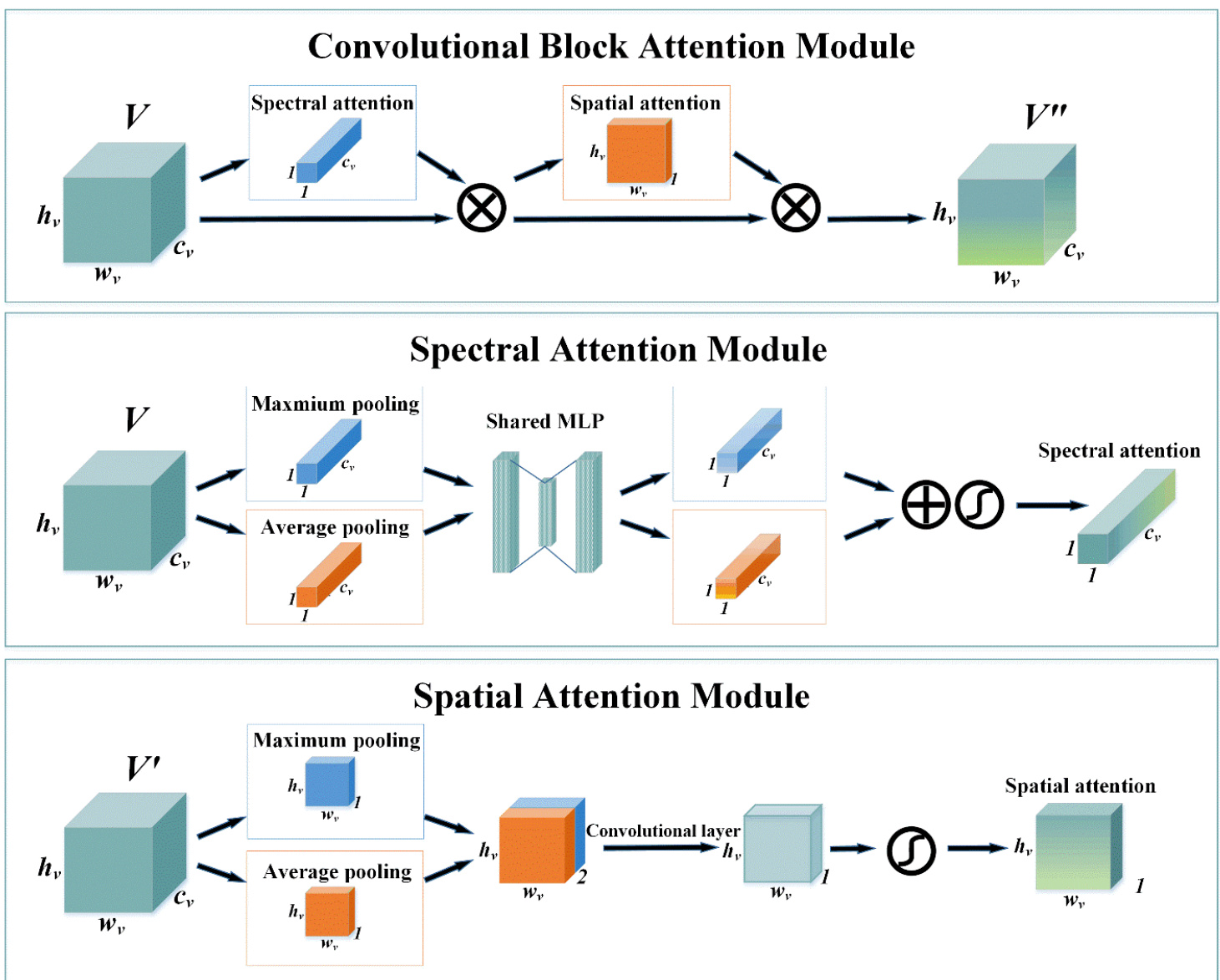
Fig. 5 The top block is the overall structure of the convolutional attention block, it consists of the spectral attention module and the spatial attention module. The middle block represents the generation of spectral attention. The bottom block denotes the generation of spatial attention.
图 5: 顶部模块展示了卷积注意力块的整体结构,由频谱注意力模块和空间注意力模块组成。中间模块表示频谱注意力的生成过程。底部模块展示了空间注意力的生成机制。
Attention-based bidirectional LSTM
基于注意力机制的双向LSTM
For each temporal slice $S_{i}\in R^{h\times w\times2f},i~=~1,2,\dots,2T$ , the final output of the attention-based CNN is $P_{i}\in R^{150}$ . Since the variation between different temporal slices contains temporal information for emotion recognition, we utilize an attentionbased bidirectional LSTM to explore the importance of different slices, as shown in Fig. 6.
对于每个时间切片 $S_{i}\in R^{h\times w\times2f},i~=~1,2,\dots,2T$ ,基于注意力机制的 CNN (Convolutional Neural Network) 最终输出为 $P_{i}\in R^{150}$ 。由于不同时间切片间的变化包含情感识别的时序信息,我们采用基于注意力的双向 LSTM (Long Short-Term Memory) 来探索不同切片的重要性,如图 6 所示。
A bidirectional LSTM connects two unidirectional LSTMs with opposite directions to the same output. Comparing with a unidirectional LSTM, a bidirectional LSTM preserves information from both past and future, making it understand the context better. In this paper, the bidirectional LSTM comprises two unidirectional LSTMs with 36 memory cells. The unidirectional LSTM for positive time direction, LSTMP takes the output sequence of the attention-based CNN $P^{P}=$ $(P_{1},P_{2},...,P_{2T})$ as the input sequence, while the other for negative time direction, ${\mathrm{LSTM}}_{\mathrm{N}}$ takes the reverse sequence
双向LSTM将两个方向相反的单向LSTM连接到同一个输出。与单向LSTM相比,双向LSTM能同时保留过去和未来的信息,从而更好地理解上下文。本文采用的双向LSTM包含两个各具36个记忆单元的单向LSTM:正向时间流的单向LSTM (LSTMP) 以注意力机制CNN的输出序列 $P^{P}=$ $(P_{1},P_{2},...,P_{2T})$ 作为输入序列,而负向时间流的 ${\mathrm{LSTM}}_{\mathrm{N}}$ 则接收逆向序列。
$P^{N}=(P_{2T},P_{2T-1},\ldots,P_{1})$ as the input sequence. The outputs of the $i{-}t h$ node of the unidirectional LSTMs are $Y_{i}^{P}\in R^{36}$ and $Y_{i}^{N}\in R^{36},i~=~1,2,\ldots,2T$ , respectively. Then, we concatenate $Y_{i}^{P}$ and $Y_{2T+1-i}^{N}$ as the output of the $i{-}t h$ node of the bidirectional LSTM $Y_{i}\in R^{72}$ . Different from traditional ways that only use the output of the last node of an LSTM for classification or other applications, we take the outputs of all the bidirectional LSTM nodes $Y\in R^{2T\times72}$ into consideration and explore the importance of different temporal slices by the temporal attention mechanism.
$P^{N}=(P_{2T},P_{2T-1},\ldots,P_{1})$ 作为输入序列。单向LSTM的第$i$个节点输出分别为$Y_{i}^{P}\in R^{36}$和$Y_{i}^{N}\in R^{36},i~=~1,2,\ldots,2T$。接着,我们将$Y_{i}^{P}$和$Y_{2T+1-i}^{N}$拼接为双向LSTM第$i$个节点的输出$Y_{i}\in R^{72}$。与传统方法仅使用LSTM末节点输出进行分类或其他应用不同,我们综合考虑所有双向LSTM节点的输出$Y\in R^{2T\times72}$,并通过时序注意力机制探索不同时间片段的重要性。
The temporal attention mechanism is implemented with two fully-connected layers, a $R e l u$ activation function, and a softmax activation function, which is defined as:
时间注意力机制通过两个全连接层、一个$ReLU$激活函数和一个softmax激活函数实现,其定义为:
$$
\begin{array}{c}{{T e m_{i}=W_{2}^{T}\Big(R e l u(W_{1}^{T}\mathrm{Y_{i}}+b_{1}^{T})\Big)+b_{2}^{T}}}\ {{A_{t e m p o r a l}=s o f t m a x(T e m)}}\ {{s o f t m a x(x)={\displaystyle\frac{e x p(x)}{\sum e x p(x)}}}}\end{array}
$$
$$
\begin{array}{c}{{T e m_{i}=W_{2}^{T}\Big(R e l u(W_{1}^{T}\mathrm{Y_{i}}+b_{1}^{T})\Big)+b_{2}^{T}}}\ {{A_{t e m p o r a l}=s o f t m a x(T e m)}}\ {{s o f t m a x(x)={\displaystyle\frac{e x p(x)}{\sum e x p(x)}}}}\end{array}
$$
where $W_{1}^{T},~W_{2}^{T},~b_{1}^{T}$ , and $b_{2}^{T}$ are learnable parameters, $T e m_{i}$ represents the $i$ -th element of $T e m\in R^{2T\times1}$ which projects $Y\in R^{2T\times72}$ to a lower dimension, and $A_{t e m p o r a l}\in R^{2T\times1}$ is the temporal attention. The elements of $A_{t e m p o r a l}$ represent the importance of the corresponding temporal slices. Subsequently, the high-level representation of the 4D sample $X_{n}$ can be defined as:
其中 $W_{1}^{T},~W_{2}^{T},~b_{1}^{T}$ 和 $b_{2}^{T}$ 是可学习参数,$T e m_{i}$ 表示将 $Y\in R^{2T\times72}$ 投影到低维空间的 $T e m\in R^{2T\times1}$ 的第 $i$ 个元素,$A_{t e m p o r a l}\in R^{2T\times1}$ 是时序注意力。$A_{t e m p o r a l}$ 的元素表示对应时间片段的重要性。随后,4D样本 $X_{n}$ 的高层表征可定义为:
$L_{n}(e)=\sum A_{t e m p o r a l}\otimes Y_{e},e=1,2,\ldots,72$ (20) where $Y_{e}\in\mathrm{R}^{2\mathrm{T}\times1}$ denotes the $e{\mathrm{-}}t h$ column of $Y\in{\mathrm{R}}^{2\mathrm{T}\times72}$ and $L_{n}(e)$ is the $e$ -th element of the high-level representation $L_{n}\in R^{72}$ , which integrates spatial, spectral, and temporal information of $X_{n}$ .
$L_{n}(e)=\sum A_{t e m p o r a l}\otimes Y_{e},e=1,2,\ldots,72$ (20) 其中 $Y_{e}\in\mathrm{R}^{2\mathrm{T}\times1}$ 表示 $Y\in{\mathrm{R}}^{2\mathrm{T}\times72}$ 的第 $e$ 列,$L_{n}(e)$ 是高层表征 $L_{n}\in R^{72}$ 的第 $e$ 个元素,该表征整合了 $X_{n}$ 的空间、光谱和时间信息。

Fig. 6 The top block is the structure of the bidirectional LSTM. We concatenate the outputs of LSTMP and LSTMP as the output of the bidirectional LSTM, $Y\in R^{2T\times72}$ . The middle block represents the projection of the outputs of the bidirectional LSTM. The bottom block denotes the generation of temporal attention.
图 6: 顶部模块展示了双向 LSTM (Long Short-Term Memory) 的结构。我们将 LSTMP 和 LSTMP 的输出拼接作为双向 LSTM 的输出 $Y\in R^{2T\times72}$。中间模块表示双向 LSTM 输出的投影过程。底部模块则展示了时序注意力 (temporal attention) 的生成机制。
Classifier
分类器
Based on the high-level representation $L_{n}$ of EEG signals, we apply a fully-connected layer and a softmax activation
基于EEG信号的高层表示$L_{n}$,我们应用了一个全连接层和一个softmax激活函数
function to predict the label of the 4D sample $X_{n}$ , which can be defined as follows:
预测4D样本$X_{n}$标签的函数可定义如下:
$$
P r e=s o f t m a x(W^{p}L_{n}+b^{p})
$$
$$
P r e=s o f t m a x(W^{p}L_{n}+b^{p})
$$
where $W^{p},b^{p}$ are learnable parameters and $P r e\in R^{C}$ denotes the probability of $X_{n}$ belonging to all the $C$ classes. Specifically, the class of the largest probability is the predicted label of 4D-aNN.
其中 $W^{p},b^{p}$ 是可学习参数,$P r e\in R^{C}$ 表示 $X_{n}$ 属于所有 $C$ 个类别的概率。具体而言,概率最大的类别即为4D-aNN的预测标签。
Experiment
实验
In this section, we firstly introduce a widely used dataset. Then, the experiment settings are described. Finally, the results on the dataset are reported and discussed.
在本节中,我们首先介绍一个广泛使用的数据集,随后说明实验设置,最后报告并讨论该数据集上的实验结果。
SEED Dataset
SEED 数据集
SEED dataset (Zheng and Lu 2015) contains 3 different categories of emotion data: positive, neutral, and negative. For each kind of emotion, 5 film clips that are about 4 minutes long and can elicit the desired target emotion are selected. 15 healthy subjects (7 males and 8 females, with age $(23.27\pm$ 2.37)) take part in the EEG signals collection experiment. 3 groups of experiments are conducted for each subject, and each experiment consists of 15 clips viewing processes. Each clip viewing process can be divided into four stages, including a 5 seconds hint of start, a 4 minutes clip period, a 45 seconds self-assessment, and a 15 seconds rest period. The order of the 15 clips is arranged so that two clips eliciting the same emotion are not shown consecutively. The EEG signals in the experiments are recorded by a 62-channel’s E I euro can system and down-sampled to $200\mathrm{Hz}$ . Besides, the EEG signals seriously contaminated by electro myo graph y (EMG) and electro o cul o graph y (EOG) are removed manually. Then, a bandpass filter between 0.3 to $50\mathrm{Hz}$ is applied to filter the noise.
SEED数据集 (Zheng and Lu 2015) 包含3种不同类别的情绪数据:积极、中性和消极。针对每种情绪,选取了5段约4分钟长且能诱发目标情绪的电影片段。15名健康受试者 (7男8女,年龄 $(23.27\pm$ 2.37)) 参与了脑电信号采集实验。每位受试者进行3组实验,每组实验包含15段视频观看流程。每段视频观看流程可分为四个阶段:5秒开始提示、4分钟视频播放、45秒自我评估和15秒休息间隔。15段视频的播放顺序经过编排,确保诱发相同情绪的视频不会连续播放。实验中的脑电信号通过62通道的E I euro can系统采集,并降采样至 $200\mathrm{Hz}$。此外,受肌电图 (EMG) 和眼电图 (EOG) 严重污染的脑电信号会被人工剔除,随后使用0.3至 $50\mathrm{Hz}$ 的带通滤波器进行噪声滤除。
Settings
设置
The proposed 4D-aNN takes a 4D segment $X_{n}\in R^{h\times w\times2f\times2T}$ as the input. In this paper, we adopt the 2D sparse map with $h=19$ and $w=19$ to maintain the positional relationship of electrodes. As shown in previous works, the combination of all the 5 bands can contribute to better results so that we set $f=5$ . For each experiment, we set the length of segments $T$ as 3, obtaining about 1128 samples per experiment. Then, we conduct a fivefold cross-validation on each experiment and calculate the average classification accuracy (ACC) and standard deviation (STD) of 3 experiments for each subject. The average ACC and STD of all subjects are taken as the final performances of our method. We train the 4D-aNN on an NVIDIA GTX 1080 GPU. The Adam optimization is applied to minimize the loss function. We set the learning rate as 0.0003, the batch size as 12, and the maximum of epochs as 150.
提出的4D-aNN以4D片段$X_{n}\in R^{h\times w\times2f\times2T}$作为输入。本文采用$h=19$和$w=19$的2D稀疏映射来保持电极位置关系。如先前工作所示,5个频段的组合能获得更好结果,因此设$f=5$。每个实验设置片段长度$T$为3,获得约1128个样本。随后对每个实验进行五折交叉验证,并计算每位受试者3次实验的平均分类准确率(ACC)和标准差(STD)。所有受试者的平均ACC与STD作为方法最终性能指标。4D-aNN在NVIDIA GTX 1080 GPU上训练,采用Adam优化器最小化损失函数,设置学习率为0.0003、批量大小为12、最大训练轮数为150。
Baseline Models
基线模型
Results
结果
We compare our model with 5 baseline models on SEED dataset. Table 1 presents the average ACC and STD of these models for EEG emotion recognition. HCNN uses the hierarchical CNN architecture to classify emotion, but only considers the spatial information of EEG signals, reaching $88.60%$ on classification accuracy. BiHDM (Li et al. 2020) applies four directed RNNs to obtain the deep representation o all the EEG electrodes’ signals, reaching $93.12%$ on classification accuracy. RGNN considers the biological topology among different brain regions, reaching $94.24%$ on classification accuracy. 4D-CRNN takes 4D DE feature maps containing spatial, spectral, and temporal information as inputs, reaching $94.74%$ on classification accuracy. SSTEmotionNet uses a two-stream network with the attention mechanisms, reaching $96.02%$ on classification accuracy. However, the data size of each input sample of SSTEmotionNet is about 4 times larger than 4D-aNN. Comparing with the baseline models, the proposed 4D-aNN achieves the state-of-the-art performance on the SEED dataset under intrasubject splitting. The average ACC of all subjects is $96.10%$ . The performances on each subject are shown as Fig. 7, and there are 9 subjects (#5, #6, #8, #9, #10, #11, #12, #13, and #15) whose performances are better than the average ACC. Specifically, to make a fair comparison with 4D-CRNN, we conduct experiments on 4D-aNN (DE) and 4D-aNN (PSD), which represents the 4D-aNN only takes DE features as inputs and only takes PSD features as inputs, respectively. The accuracy of 4D-aNN (DE) exceeds that of 4D-CRNN by $0.65%$ , indicating the superiority of the proposed 4D-aNN. When compared with 4D-aNN (DE) and 4D-aNN (PSD), 4DaNN displays the best performance, which indicates the effectiveness of the combination of different features.
我们在SEED数据集上将模型与5个基线模型进行了比较。表1展示了这些模型在EEG情绪识别任务上的平均准确率(ACC)和标准差(STD)。HCNN采用分层CNN架构进行情绪分类,但仅考虑EEG信号的空间信息,分类准确率达到88.60%。BiHDM (Li et al. 2020)应用四个定向RNN来获取所有EEG电极信号的深层表征,分类准确率达到93.12%。RGNN考虑了不同脑区之间的生物拓扑结构,分类准确率达到94.24%。4D-CRNN以包含空间、频谱和时间信息的4D微分熵(DE)特征图作为输入,分类准确率达到94.74%。SSTEmotionNet采用带有注意力机制的双流网络,分类准确率达到96.02%。然而,SSTEmotionNet每个输入样本的数据量约为4D-aNN的4倍。与基线模型相比,提出的4D-aNN在受试者内划分条件下在SEED数据集上达到了最先进的性能,所有受试者的平均ACC为96.10%。各受试者的表现如图7所示,其中9位受试者(#5、#6、#8、#9、#10、#11、#12、#13和#15)的表现优于平均ACC。特别地,为与4D-CRNN进行公平比较,我们分别对仅使用DE特征输入的4D-aNN(DE)和仅使用功率谱密度(PSD)特征输入的4D-aNN(PSD)进行了实验。4D-aNN(DE)的准确率比4D-CRNN高出0.65%,证明了所提4D-aNN的优越性。与4D-aNN(DE)和4D-aNN(PSD)相比,4D-aNN展现出最佳性能,这表明不同特征组合的有效性。
Table 1 The performance (average ACC and STD $(%).$ of the compared models.
表 1: 对比模型的性能 (平均准确率 ACC 和标准差 STD $(%).$
| 模型 | SEED |
|---|---|
| ACC (%) | |
| HCNN (Li et al. 2018) | 88.60 |
| BiHDM (Li et al. 2020) | 93.12 |
| RGNN (Zhong et al. 2020) | 94.24 |
| 4D-CRNN (Shen et al. 2020) | 94.74 |
| SST-EmotionNet (Jia et al. 2020) | 96.02 |
| 4D-aNN | 96.10 |
| 4D-aNN (DE) | 95.39 |
| 4D-aNN (PSD) | 90.49 |

Fig. 7 The performance of 4D-aNN on each subject. In the SEED dataset, 3 experiments are conducted for each subject. We evaluate the performance of each experiment and also present the average classification accuracy for each subject.
图 7: 4D-aNN 在各被试上的性能表现。在 SEED 数据集中,每位被试进行 3 次实验。我们评估了每次实验的性能,并给出了每位被试的平均分类准确率。
To verify the importance of the attention mechanisms in our model, we conduct an additional experiment for ablation studies on SEED dataset. The experiment is ablation on spatial, spectral, and temporal attention mechanisms. We evaluate the performances of 4D-aNN when spatial, spectral, temporal, and all the attention mechanisms are ablated respectively. As shown in Fig. 8, when one of the attention mechanisms is ablated, the classification accuracy decreases. 4D-aNN without the spectral attention mechanism decreases by $0.63%$ , 4D-aNN without the spatial attention mechanism decreases by $0.47%$ , and 4D-aNN without the temporal attention mechanism decrease by $1.19%$ . Specifically, 4D-aNN without all the attention mechanisms decreases by $2.17%$ , which is the worst among the models used for comparison. In conclusion, the results indicate that the attention mechanisms make contributions to EEG emotion recognition for the ability to capture the disc rim i native local patterns in spatial, spectral, and temporal domains.
为验证注意力机制在我们模型中的重要性,我们在SEED数据集上进行了消融实验。该实验针对空间、频谱和时间注意力机制进行消融研究。我们分别评估了当空间、频谱、时间以及全部注意力机制被移除时4D-aNN的性能表现。如图8所示,当任一注意力机制被移除时,分类准确率均出现下降:移除频谱注意力机制的4D-aNN下降$0.63%$,移除空间注意力机制的下降$0.47%$,移除时间注意力机制的下降$1.19%$。特别值得注意的是,移除全部注意力机制的4D-aNN准确率下降达$2.17%$,在所有对比模型中表现最差。实验结果表明,注意力机制通过捕捉空间、频谱和时间域中的判别性局部模式,对脑电情绪识别任务具有重要贡献。

Fig. 8 Ablation studies on different input features and attention modules of 4D-a . “−” denotes the a lation on certain attention modules.
图 8: 4D-a 不同输入特征和注意力模块的消融研究。"−"表示对特定注意力模块的消融。
In particular, to explore the critical brain regions for different emotions, we separately depict the electrode activity heatmaps in Fig. 9. We draw the heatmaps using Grad $C A M{+}{+}$ (Chat to pad hay et al. 2018), based on the experimental results of subject 15. Grad $C A M{+}{+}$ uses the last convolutional layer feature maps and the class scores of the classifier to generate heatmaps. The heatmaps are able to explain which input regions are important for predictions. In this work, the size of each heatmap is $19\times19$ , which is the same as the 2D sparse map. The elements in the heatmaps represent the contributions of the corresponding brain regions to the recognition of the target emotions. From Fig. 9, We can observe the distinct distributions of important brain regions with regard to different emotions: channels FC5, FC3, and $C5$ are important for recognition of positive emotions, channels CP5, CP3, and $C P I$ are important for recognition of neutral emotions, and channels $P O7,P O5$ , and $P3$ are important for recognition of negative emotions for subject #15. In particular, the critical brain regions could vary with different subjects, time, and emotions so that the attention mechanisms that enable 4D-aNN to adaptively capture disc rim i native patterns make sense for EEG emotion recognition.
特别是为了探索不同情绪对应的关键脑区,我们在图9中分别绘制了电极活动热力图。这些热力图基于受试者#15的实验结果,采用Grad $C A M{+}{+}$ (Chat to pad hay et al. 2018)方法绘制。Grad $C A M{+}{+}$ 利用最后一个卷积层的特征图与分类器的类别分数生成热力图,能够解释哪些输入区域对预测结果具有重要性。本研究中,每张热力图尺寸为$19\times19$,与二维稀疏图保持一致。热力图中各元素代表对应脑区对目标情绪识别的贡献度。
从图9可以观察到,不同情绪的重要脑区分布存在显著差异:对于受试者15而言,通道FC5、FC3和$C5$对积极情绪识别至关重要,通道CP5、CP3和$C P I$对中性情绪识别起关键作用,而通道$P O7$、$P O5$和$P3$则主导了消极情绪的识别。值得注意的是,关键脑区可能随受试者个体、时间及情绪类型动态变化,因此4D-aNN通过注意力机制自适应捕捉判别性模式的设计,对脑电情绪识别具有重要价值。

Fig. 9 The electrode activity heatmaps based on the experimental results of subject $#15$ Parts (a), (b), and (c) correspond to positive, neutral, and negative emotions, respectively. Dark red regions denote more significant contributions to the recognition of the corresponding emotions.
图 9: 基于受试者 $#15$ 实验结果的电极活动热图 (a) 、(b) 和 (c) 部分分别对应积极、中性和消极情绪。深红色区域表示对相应情绪识别有更显著贡献。
Discussion
讨论
We conduct several experiments to investigate the use of 4D-aNN which fuses the spatial-spectral-temporal information and the effectiveness of the attention mechanisms on different domains for EEG emotion classification. In this section, we discuss three noteworthy points.
我们进行了多项实验,研究利用融合空间-光谱-时间信息的4D-aNN以及注意力机制在不同领域对EEG情绪分类的有效性。本节将讨论三个值得注意的要点。
First, to deal with the spatial-spectral information, we apply an attention-based CNN which consists of a CNN network, a spectral attention module, and a spatial attention module. The CNN network extracts the spatial-spectral representation from inputs first. Then, the spectral attention mechanism is applied to each spectral feature to explore the importance of different frequency bands and features. Besides, the spatial attention mechanism is applied to each 2D feature map to adaptively capture the critical brain regions. The critical brain regions and frequency bands could vary with different individuals, emotions, and time so that the ability to capture disc rim i native patterns of the attention modules improves the performance of 4D-aNN.
首先,为处理空间-频谱信息,我们采用了基于注意力机制的CNN网络,该网络由CNN主干、频谱注意力模块和空间注意力模块组成。CNN主干首先从输入数据中提取空间-频谱特征表示。随后,频谱注意力机制作用于每个频谱特征,以探索不同频段及特征的重要性。此外,空间注意力机制应用于每个二维特征图,自适应捕捉关键脑区。由于关键脑区与频段会随个体、情绪和时间动态变化,注意力模块对判别性特征的捕捉能力显著提升了4D-aNN的性能。
Second, to explore the temporal dependencies in 4D spatialspectral-temporal representations, we utilize an attentionbased bidirectional LSTM. The bidirectional LSTM extracts high-level representations from the outputs of the attentionbased CNN. Different from traditional ways that only use the output of the last node of an LSTM for classifications or other applications, we consider outputs of all the nodes with the temporal attention mechanism. The temporal attention mechanism adaptively assigns weights of different temporal slices so that the dynamic content of emotions in 4D representations could be captured better.
其次,为了探索4D空间-光谱-时间表征中的时间依赖性,我们采用了基于注意力机制的双向LSTM。该双向LSTM从基于注意力的CNN输出中提取高级表征。与传统仅使用LSTM最后一个节点输出进行分类或其他应用的方式不同,我们通过时序注意力机制综合考虑所有节点的输出。该时序注意力机制能自适应地为不同时间切片分配权重,从而更精准捕捉4D表征中情绪内容的动态变化。
Third, to address the importance of the attention mechanisms, we conduct ablation studies on different attention modules. 4D-aNN without the spatial, spectral, and temporal attention mechanism decreases by $0.47%$ , $0.63%$ , and $1.19%$ on classification accuracy, respectively. In particular, 4D-aNN without all the attention mechanisms decreases by $2.17%$ , which is the worst among the models in comparison. The experimental results demonstrate the effectiveness of the attention mechanisms to adaptively capture disc rim i native patterns.
第三,为了验证注意力机制的重要性,我们对不同注意力模块进行了消融实验。移除空间、光谱和时间注意力机制的4D-aNN在分类准确率上分别下降了$0.47%$、$0.63%$和$1.19%$。特别值得注意的是,移除所有注意力机制的4D-aNN性能下降了$2.17%$,这是对比模型中表现最差的。实验结果证明了注意力机制在自适应捕捉判别性模式方面的有效性。
Conclusion
结论
In this paper, we propose the 4D-aNN model for EEG emotion recognition. The 4D-aNN takes 4D spatial-spectraltemporal representations containing spatial, spectral, and temporal information of EEG signals as inputs. We integrate the attention mechanisms into the CNN module and the bidirectional LSTM module. The CNN module deals with the spatial and spectral information of EEG signals while the spatial and spectral attention mechanisms capture critical brain regions and frequency bands adaptively. The bidirectional LSTM module extracts temporal dependencies on the outputs of the CNN module while the temporal attention mechanism explores the importance of different temporal slices. The experiments on SEED dataset demonstrate better performance than all baselines. In particular, the ablation studies on different attention modules show the effectiveness of the attention mechanisms in our model for EEG emotion recognition.
本文提出用于脑电图(EEG)情绪识别的4D-aNN模型。该模型以包含EEG信号空间、频谱和时间信息的4D空间-频谱-时序表征作为输入。我们将注意力机制分别集成到CNN模块和双向LSTM模块中:CNN模块处理EEG信号的空间与频谱信息,同时通过空间注意力与频谱注意力机制自适应捕获关键脑区与频段;双向LSTM模块提取CNN模块输出的时序依赖关系,并通过时间注意力机制探索不同时间片段的重要性。在SEED数据集上的实验表明,本模型性能优于所有基线方法。特别地,针对不同注意力模块的消融研究验证了注意力机制在EEG情绪识别模型中的有效性。