CUT YOUR LOSSES IN LARGE-VOCABULARY LANGUAGE MODELS
在大词汇量语言模型中减少损失
Erik Wijmans∗Brody Huval Alexander Hertzberg Vladlen Koltun Philipp Kra¨henbu¨hl Apple
Erik Wijmans∗Brody Huval Alexander Hertzberg Vladlen Koltun Philipp Kra¨henbu¨hl Apple
ABSTRACT
摘要
As language models grow ever larger, so do their vocabularies. This has shifted the memory footprint of LLMs during training disproportionately to one single layer: the cross-entropy in the loss computation. Cross-entropy builds up a logit matrix with entries for each pair of input tokens and vocabulary items and, for small models, consumes an order of magnitude more memory than the rest of the LLM combined. We propose Cut Cross-Entropy (CCE), a method that computes the cross-entropy loss without materializing the logits for all tokens into global memory. Rather, CCE only computes the logit for the correct token and evaluates the log-sum-exp over all logits on the fly. We implement a custom kernel that performs the matrix multiplications and the log-sum-exp reduction over the vocabulary in flash memory, making global memory consumption for the cross-entropy computation negligible. This has a dramatic effect. Taking the Gemma 2 (2B) model as an example, CCE reduces the memory footprint of the loss computation from $24:\mathrm{GB}$ to 1 MB, and the total training-time memory consumption of the classifier head from 28 GB to 1 GB. To improve the throughput of CCE, we leverage the inherent sparsity of softmax and propose to skip elements of the gradient computation that have a negligible (i.e., below numerical precision) contribution to the gradient. Experiments demonstrate that the dramatic reduction in memory consumption is accomplished without sacrificing training speed or convergence.
随着语言模型规模的不断扩大,其词汇量也在增长。这导致了大语言模型在训练过程中,内存占用不均衡地集中在某一个层上:损失计算中的交叉熵。交叉熵会构建一个 logit 矩阵,其中包含每对输入 token 和词汇项的条目,对于小模型而言,其占用的内存比大语言模型其余部分的总和还要多一个数量级。我们提出了 Cut Cross-Entropy (CCE) 方法,该方法在计算交叉熵损失时,不会将所有 token 的 logit 存储到全局内存中。相反,CCE 仅计算正确 token 的 logit,并即时评估所有 logit 的 log-sum-exp。我们实现了一个自定义内核,该内核在闪存中执行矩阵乘法和词汇表的 log-sum-exp 归约,使得交叉熵计算的全局内存消耗可以忽略不计。这带来了显著的效果。以 Gemma 2 (2B) 模型为例,CCE 将损失计算的内存占用从 $24:\mathrm{GB}$ 减少到 1 MB,分类器头在训练期间的总内存消耗从 28 GB 减少到 1 GB。为了提高 CCE 的吞吐量,我们利用了 softmax 的固有稀疏性,并建议跳过对梯度贡献可以忽略不计(即低于数值精度)的梯度计算元素。实验表明,内存消耗的显著减少并未牺牲训练速度或收敛性。
1 INTRODUCTION
1 引言
Progress in large language models (LLMs) has been fueled in part by an increase in parameter count, context length, and vocabulary size (the number of tokens that can be used to represent the input). As LLMs grew, so did the associated infrastructure. Large mini-batch gradient descent (Goyal et al., 2017) combined with data-parallelism (Hillis & Steele, 1986) enabled the harnessing of increasing computational power. ZeRO (Raj bh and ari et al., 2020) broke the dependence between the number of GPUs and the memory used for model parameters, gradients, and optimizer state. Activation check pointing (Chen et al., 2016) reduced the amount of memory used for activation s, supporting the development of deeper models. Flash Attention (Dao et al., 2022) reduced the memory used in selfattention from $O(N^{\bar{2}})$ to $O(N)$ , thereby supporting longer context windows. These improvements gradually shifted the memory consumption of LLM training to one single layer – the cross-entropy loss, whose memory footprint grows with the product of vocabulary size and number of tokens per batch. The cross-entropy loss is responsible for up to $90%$ of the memory footprint of modern LLM training (see Fig. 1a). The problem grows only more acute with time, since even the largest contemporary vocabularies (e.g., 256K tokens) may benefit from further expansion (Tao et al., 2024).
大语言模型 (LLM) 的进展部分得益于参数数量、上下文长度和词汇表大小(可用于表示输入的 Token 数量)的增加。随着大语言模型的增长,相关基础设施也随之发展。大 mini-batch 梯度下降 (Goyal et al., 2017) 结合数据并行 (Hillis & Steele, 1986) 使得计算能力的利用得以增强。ZeRO (Rajbh and ari et al., 2020) 打破了 GPU 数量与模型参数、梯度和优化器状态内存使用之间的依赖关系。激活检查点 (Chen et al., 2016) 减少了激活内存的使用,支持更深层模型的开发。Flash Attention (Dao et al., 2022) 将自注意力机制的内存使用从 $O(N^{\bar{2}})$ 降低到 $O(N)$ ,从而支持更长的上下文窗口。这些改进逐渐将大语言模型训练的内存消耗转移到单一层——交叉熵损失,其内存占用随着词汇表大小和每批次 Token 数量的乘积增长。现代大语言模型训练中,交叉熵损失占内存占用的高达 $90%$ (见图 1a)。随着时间的推移,问题只会变得更加严重,因为即使是当今最大的词汇表(例如 256K Token)也可能受益于进一步扩展 (Tao et al., 2024)。
We propose a cross-entropy implementation, Cut Cross-Entropy (CCE), that has a negligible memory footprint and scales to arbitrarily large vocabularies. Our key insight is that computation of the loss and its gradient only depends on a single log-probability, that of the ground-truth label. With an arithmetic reformulation, we decompose the cross-entropy loss into an index matrix multiplication over a single ground-truth label and a log-sum-exp operation over all vocabulary entries for each token. Each operation has small and well-defined inputs – the network embeddings and classifier
我们提出了一种交叉熵的实现方法,称为Cut Cross-Entropy (CCE),它具有可忽略的内存占用,并且可以扩展到任意大的词汇量。我们的关键洞察是,损失及其梯度的计算仅依赖于单个对数概率,即真实标签的概率。通过算术重构,我们将交叉熵损失分解为单个真实标签的索引矩阵乘法和对每个Token的所有词汇表条目进行的log-sum-exp操作。每个操作都有小而明确的输入——网络嵌入和分类器。

Figure 1: Memory use and maximum attainable batch size (in millions of tokens) for a variety of frontier models on a 16-GPU (80 GB each) fully-sharded data-parallel setup (Rajbhandari et al., 2020) with activation check pointing (Chen et al., 2016) and a mixed-precision 16-bit (fp16/bf16) AdamW optimizer (Kingma & Ba, 2015; Loshchilov & Hutter, 2019). For each model, we break its memory use down into weights and optimizer states, activation checkpoints, and the log-probabilities computed by the cross-entropy loss layer. Our Cut Cross-Entropy (CCE) enables increasing the batch size by $1.5\mathrm{x}$ (Llama 2 13B) to 10x (GPT 2, Gemma 2 2B), with no sacrifice in speed or convergence. Exact values in Table A3.
图 1: 在 16-GPU(每个 80 GB)全分片数据并行设置(Rajbhandari 等人, 2020)上,使用激活检查点(Chen 等人, 2016)和混合精度 16 位(fp16/bf16)AdamW 优化器(Kingma & Ba, 2015; Loshchilov & Hutter, 2019)的各种前沿模型的内存使用和最大可达到的批次大小(以百万 token 计)。对于每个模型,我们将其内存使用分解为权重和优化器状态、激活检查点以及由交叉熵损失层计算的对数概率。我们的 Cut Cross-Entropy (CCE) 使得批次大小增加了 $1.5\mathrm{x}$(Llama 2 13B)到 10x(GPT 2, Gemma 2 2B),且没有牺牲速度或收敛性。具体值见表 A3。
matrix – and a single scalar output per token. Both operations do, however, rely on a large intermediate logit matrix that computes the score for each token and potential vocabulary entry. We show that there is no need to materialize this logit matrix in GPU memory. Instead, we compute logits as needed in SRAM in a series of custom CUDA kernels. The result is a cross-entropy computation that has negligible memory footprint, with no detrimental effect on latency or convergence. See Fig. 1b for a breakdown of memory savings and consequent batch size increases afforded by CCE.
矩阵——以及每个Token的单个标量输出。然而,这两种操作都依赖于一个大的中间logit矩阵,该矩阵计算每个Token和潜在词汇表项的分数。我们展示了无需在GPU内存中物化这个logit矩阵。相反,我们在SRAM中按需计算logits,通过一系列定制的CUDA内核。结果是交叉熵计算的内存占用可以忽略不计,对延迟或收敛没有负面影响。有关CCE节省的内存和由此带来的批量大小增加的详细分解,请参见图1b。
2 RELATED WORK
2 相关工作
Attention mechanisms. The effectiveness of transformers (Vaswani et al., 2017) in modeling language has drawn attention to their compute and memory requirements. Multiple works have proposed alternatives to scaled dot-product attention that reduce transformers’ computation and memory (Kitaev et al., 2020; Wang et al., 2020; Cho roman ski et al., 2021). Other model classes, such as structured state-space models (Gu et al., 2022; Gu & Dao, 2023), have also shown promising results. We study a different part of the model – its classifier head – that is not considered in these works.
注意力机制。Transformer(Vaswani 等, 2017)在语言建模中的有效性引发了对其计算和内存需求的关注。多项研究提出了替代缩放点积注意力的方法,以减少 Transformer 的计算和内存消耗(Kitaev 等, 2020; Wang 等, 2020; Choromanski 等, 2021)。其他模型类别,如结构化状态空间模型(Gu 等, 2022; Gu & Dao, 2023),也展示了有前景的结果。我们研究了模型的一个不同部分——其分类器头——这些工作并未涉及。
Attention implementations. In addition to alternative attention mechanisms, the community has also tackled the daunting memory consumption of LLMs via efficient implementations. Rabe & Staats (2021) developed a self-attention implementation that makes use of chunking. Chen et al. (2023) proposed an implementation that broke the operation into two stages, reduction and matrix multiplication. This makes efficient use of GPU memory and registers but requires re computation in the forward pass. Flash Attention (Dao et al., 2022) uses an online softmax (Milakov & Gimelshein, 2018) and, like CCE, materializes blocks of the $N^{2}$ -sized self-attention matrix in on-chip SRAM rather than slower global DRAM. This is one of the key ideas that CCE builds on to develop a memory-efficient cross-entropy formulation.
注意力机制实现。除了替代的注意力机制外,社区还通过高效实现解决了大语言模型令人望而生畏的内存消耗问题。Rabe & Staats (2021) 开发了一种利用分块的自注意力实现。Chen 等 (2023) 提出了一种将操作分为两个阶段的实现,即归约和矩阵乘法。这使得 GPU 内存和寄存器的使用更加高效,但需要在正向传播时重新计算。Flash Attention (Dao 等, 2022) 使用了在线 softmax (Milakov & Gimelshein, 2018),并且与 CCE 类似,它将大小为 $N^{2}$ 的自注意力矩阵块实现在片上 SRAM 中,而不是较慢的全局 DRAM 中。这是 CCE 开发内存高效交叉熵公式的关键思想之一。
Vocabulary reduction. One way to minimize the amount of memory used by the log-probabilities over the tokens is to reduce the number of ‘active’ tokens in the vocabulary. Grave et al. (2017) proposed to use a vocabulary with a hierarchical structure, thereby requiring the log-probabilities for only a subset of the vocabulary at any given time. Yu et al. (2023) explore token iz ation-free byte-level models that operate on dramatically smaller vocabularies.
词汇缩减。一种减少对 Token 的对数概率所占内存的方法是通过减少词汇表中“活跃” Token 的数量。Grave 等人 (2017) 提出使用具有层次结构的词汇表,从而在任何给定时间只需要词汇表中一部分的对数概率。Yu 等人 (2023) 探索了基于字节级别的无 Token 化模型,这些模型在显著更小的词汇表上运行。
Efficient cross-entropy implementations. A number of recent implementations use chunking to reduce the memory usage of the cross-entropy layer. Yet chunking induces a trade-off. Memory footprint is minimized when the number of chunks is high, but latency is minimized when the number of chunks is low. CCE utilizes only on-chip SRAM and minimizes both memory footprint and latency. Liger Kernels (Hsu et al., 2024) make efficient use of the GPU via chunking and by computing the loss+gradient simultaneously. The latter requires that any transform applied to the loss (such as masking) is implemented in the kernel itself. CCE has separate forward and backward stages, enabling user-defined transformations on the loss.
高效的交叉熵实现。一些最近的实现使用分块来减少交叉熵层的内存使用。然而,分块会带来权衡。当分块数量较多时,内存占用最小化,但当分块数量较少时,延迟最小化。CCE 仅使用片上 SRAM,并最小化内存占用和延迟。Liger Kernels (Hsu et al., 2024) 通过分块和同时计算损失+梯度来高效利用 GPU。后者要求对损失应用的任何变换(如掩码)在内核本身中实现。CCE 具有独立的前向和后向阶段,支持用户对损失进行自定义变换。
3 PRELIMINARIES
3 预备知识
Let $\begin{array}{r}{P(x),=,\prod_{i=1}^{N}P(x_{i}\mid x_{1}\dots x_{i-1})}\end{array}$ be a Large Language Model (LLM) over a vocabulary $V$ . The LLM pa ra meterizes an auto regressive distribution over all possible tokens $x_{i}\in V$ given the preceding $N-1$ tokens. Specifically, this distribution is the combination of a backbone network $f:x_{1}\ldots x_{i-1}\to\mathbb{R}^{D}$ and a linear classifier $\mathbf{C}\in\mathbb{R}^{D\times|V|}$ :
设 $\begin{array}{r}{P(x),=,\prod_{i=1}^{N}P(x_{i}\mid x_{1}\dots x_{i-1})}\end{array}$ 为词汇表 $V$ 上的大语言模型 (LLM)。该大语言模型参数化了在给定前 $N-1$ 个 Token 的情况下,对所有可能的 Token $x_{i}\in V$ 的自回归分布。具体来说,该分布是骨干网络 $f:x_{1}\ldots x_{i-1}\to\mathbb{R}^{D}$ 和线性分类器 $\mathbf{C}\in\mathbb{R}^{D\times|V|}$ 的组合:
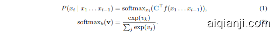
The backbone network $f(x_{1},\dots,x_{i-1})\ \in\ \mathbb{R}^{D}$ encodes a token sequence in the $D$ -dimensional feature vector. The linear classifier $\mathrm{C}\in\mathbb{R}^{D\times|V|}$ projects the embedding into an output space of the vocabulary $V$ . The $\mathrm{softmax}{k}(\mathbf{v})$ produces the probability over all vocabulary entries from the un normalized log probabilities (logits) produced by $\mathbf{C}^{\top}f(x{1}\ldots{x_{i-1}})$ .
骨干网络 $f(x_{1},\dots,x_{i-1})\ \in\ \mathbb{R}^{D}$ 将 token 序列编码为 $D$ 维特征向量。线性分类器 $\mathrm{C}\in\mathbb{R}^{D\times|V|}$ 将嵌入投影到词汇表 $V$ 的输出空间中。$\mathrm{softmax}{k}(\mathbf{v})$ 从 $\mathbf{C}^{\top}f(x{1}\ldots{x_{i-1}})$ 生成的非归一化对数概率 (logits) 生成所有词汇条目的概率。
3.1 VOCABULARY
3.1 词汇
LLMs represent their input (and output) as a set of tokens in a vocabulary $V$ . The vocabulary is typically constructed by a method such as Byte Pair Encoding (BPE) (Gage, 1994). BPE initializes the vocabulary with all valid byte sequences from a standard text encoding, such as utf-8. Then, over a large corpus of text, BPE finds the most frequent pair of tokens and creates a new token that represents this pair. This continues iterative ly until the maximum number of tokens is reached.
大语言模型将输入(和输出)表示为词汇表 $V$ 中的一组 Token。词汇表通常通过诸如字节对编码(Byte Pair Encoding, BPE)(Gage, 1994) 的方法构建。BPE 使用标准文本编码(如 utf-8)中的所有有效字节序列初始化词汇表。然后,在一个大型文本语料库中,BPE 找到最频繁出现的 Token 对,并创建一个代表该对的新 Token。这个过程会迭代进行,直到达到最大 Token 数量。
Large vocabularies enable a single token to represent multiple characters. This reduces the length of both input and output sequences, compresses larger and more diverse documents into shorter context windows, thus improving the model’s comprehension while reducing computational demands.
大词汇表使得单个 Token 能够表示多个字符。这减少了输入和输出序列的长度,将更大且更多样的文档压缩到更短的上下文窗口中,从而在减少计算需求的同时提升模型的理解能力。
3.2 INFERENCE AND TRAINING
3.2 推理与训练
Even with a large vocabulary, sampling from an LLM is memory-efficient at inference time. Specifically, the LLM produces one token at a time, computing $P(x_{i}|x_{1}\ldots x_{i-1})$ and sampling from this distribution (Kwon et al., 2023). Because the distribution over the vocabulary is only needed for a single token at a time, the memory footprint is independent of sequence length.
即使拥有较大的词汇表,从大语言模型中进行采样在推理时也是内存高效的。具体来说,大语言模型一次生成一个 Token,计算 $P(x_{i}|x_{1}\ldots x_{i-1})$ 并从这个分布中进行采样 (Kwon et al., 2023)。由于每次只需要对一个 Token 的词汇分布进行计算,因此内存占用与序列长度无关。
At training time, the LLM maximizes the log-likelihood of the next token:
在训练时,大语言模型最大化下一个 Token 的对数似然:
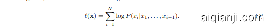
Due to the structure of most backbones (Vaswani et al., 2017; Gu et al., 2022; Gu & Dao, 2023), $f(x_{1}),f(x_{1},x_{2}),\dots,f(x_{1},\dots,x_{N})$ is efficiently computed in parallel. However, activation s for non-linear layers have to be saved for the backward pass, consuming significant memory. Most LLM training frameworks make use of aggressive activation check pointing (Chen et al., 2016), sharding (Raj bh and ari et al., 2020), and specialized attention implementations (Dao et al., 2022) to keep this memory footprint manageable.
由于大多数主干网络的结构 (Vaswani et al., 2017; Gu et al., 2022; Gu & Dao, 2023) ,$f(x_{1}),f(x_{1},x_{2}),\dots,f(x_{1},\dots,x_{N})$ 可以高效地并行计算。然而,非线性层的激活值必须保存以便反向传播,这会消耗大量内存。大多数大语言模型训练框架通过使用激进的激活检查点 (Chen et al., 2016) 、分片 (Rajbh and ari et al., 2020) 和专门的注意力实现 (Dao et al., 2022) 来保持内存占用的可管理性。
With the aforementioned optimization s, the final (cross-entropy loss) layer of the LLM becomes by far the biggest memory hog. For large vocabularies, the final cross-entropy layer accounts for the majority of the model’s memory footprint at training time (Fig. 1a). For example, the logprobabilities materialized by the cross-entropy layer account for $40\bar{%}$ of the memory consumption of Phi 3.5 (Mini) (Abdin et al., 2024) $(|V|=32,\mathrm{\dot{0}64})$ , $65%$ of the memory consumption of Llama
通过上述优化,大语言模型的最终(交叉熵损失)层成为目前最大的内存消耗者。对于大型词汇表,最终的交叉熵层在训练时占据了模型内存占用的主要部分(图 1a)。例如,由交叉熵层生成的 log 概率占据了 Phi 3.5 (Mini)(Abdin 等,2024)内存消耗的 $40\bar{%}$ $(|V|=32,\mathrm{\dot{0}64})$,以及 Llama 内存消耗的 $65%$。

Figure 2: Access patterns and computation of blockwise (a) indexed matrix multiplication, (b) linear-log-sum-exp forward pass, and (c) linear-log-sum-exp backward pass. See Algorithms 1 to 3 for the corresponding algorithms.
图 2: 分块 (a) 索引矩阵乘法, (b) 线性-log-sum-exp 前向传播, 和 (c) 线性-log-sum-exp 反向传播的访问模式和计算。相关算法参见算法 1 到 3。
3 (8B) (Dubey et al., 2024) $(|V|,=,128{,}000)$ , and $89%$ of the memory consumption of Gemma 2 (2B) (Rivie`re et al., 2024) $\mathit{\dot{\left|V\right|}},=,256{,}128)$ . In fact, the log-probabilities of Gemma 2 (2B) for a single sequence x with length $N=80{,}000$ use the entire available memory of an 80 GB H100 GPU. (The sequence length is a factor due to the use of teacher forcing for parallelism.)
3 (8B) (Dubey et al., 2024) $(|V|,=,128{,}000)$,以及 Gemma 2 (2B) (Rivie`re et al., 2024) $\mathit{\dot{\left|V\right|}},=,256{,}128)$ 的 $89%$ 内存消耗。事实上,Gemma 2 (2B) 对长度为 $N=80{,}000$ 的单个序列 x 的对数概率使用了 80 GB H100 GPU 的整个可用内存。(由于使用教师强制进行并行化,序列长度是一个因素。)
We show that a reformulation of the training objective leads to an implementation that has negligible memory consumption above what is required to store the loss and the gradient.
我们展示了重新制定训练目标后,实现的内存消耗几乎可以忽略不计,仅需存储损失和梯度所需的内存。
4 CUT CROSS-ENTROPY
4 切割交叉熵 (Cut Cross-Entropy)
Consider the cross-entropy loss $\ell_{i}$ over a single prediction of the next token $P(x_{i}|x_{1}\ldots x_{i-1})$ :
考虑下一个 Token $P(x_{i}|x_{1}\ldots x_{i-1})$ 的单个预测的交叉熵损失 $\ell_{i}$:

Here the first term is a vector product over $D$ -dimensional embeddings $E_{i}=f(x_{1}\ldots x_{i-1})$ and a classifier C. The second term is a log-sum-exp operation and is independent of the next token $x_{i}$ . During training, we optimize all next-token predictions $\pmb{\ell}=[\boldsymbol{\ell}_{1}\ldots\boldsymbol{\ell}_{N}]$ jointly using teacher forcing:
这里的第一项是 $D$ 维嵌入 $E_{i}=f(x_{1}\ldots x_{i-1})$ 和分类器 C 的向量积。第二项是对数和指数运算,与下一个token $x_{i}$ 无关。在训练过程中,我们使用教师强制联合优化所有下一个token的预测 $\pmb{\ell}=[\boldsymbol{\ell}_{1}\ldots\boldsymbol{\ell}_{N}]$:

where $\mathbb{E}=[E_{1},.,.,.,E_{N}]$ and $\left(\mathbf{C}^{\top}\mathbb{E}\right)_{\mathbf{x}}=\left[C_{x_{1}}^{\top}E_{1}\ldots C_{x_{N}}^{\top}E_{N}\right]$ . The first term in Equation (4) is a combination of an indexing operation and matrix multiplication. It has efficient forward and backward passes, in terms of both compute and memory, as described in Section 4.1. The second term in Equation (4) is a joint log-sum-exp and matrix multiplication operation. Section 4.2 describes how to compute the forward pass of this linear-log-sum-exp operation efficiently using a joint matrix multiplication and reduction kernel. Section 4.3 describes how to compute its backward pass efficiently by taking advantage of the sparsity of the gradient over a large vocabulary. Putting all the pieces together yields a memory-efficient low-latency cross-entropy loss.
其中 $\mathbb{E}=[E_{1},.,.,.,E_{N}]$ 且 $\left(\mathbf{C}^{\top}\mathbb{E}\right)_{\mathbf{x}}=\left[C_{x_{1}}^{\top}E_{1}\ldots C_{x_{N}}^{\top}E_{N}\right]$。方程 (4) 中的第一项是索引操作和矩阵乘法的组合。如第4.1节所述,它在计算和内存方面都具有高效的前向和后向传递。方程 (4) 中的第二项是联合的 log-sum-exp 和矩阵乘法操作。第4.2节描述了如何使用联合矩阵乘法和归约内核高效计算该线性-log-sum-exp操作的前向传递。第4.3节描述了如何通过利用大词汇表上梯度的稀疏性来高效计算其后向传递。将所有部分结合起来,就得到了内存高效、低延迟的交叉熵损失。
4.1 MEMORY-EFFICIENT INDEXED MATRIX MULTIPLICATION
4.1 内存高效的索引矩阵乘法
A naive computation of indexed matrix multiplication involves either explicit computation of the logits $\mathbf{C}^{\top}\mathbf{E}$ with an $O(N|V|)$ memory cost, or indexing into the classifier $\operatorname{C}{\mathbf{x}}=[C{x_{1}},.,.,.,C_{x_{N}}]$ with an $O(N D)$ memory cost. Our implementation fuses the classifier indexing $\mathbf{C_{x}}$ with the consecutive dot product between columns $C_{x_{i}}$ and $E_{i}$ in a single CUDA/Triton kernel (Tillet et al., 2019). Our kernel retrieves the value $x_{i}$ , the $x_{i}$ -th column from $\mathbf{C}$ , and the $i$ -th column from $\mathbf{E}$ , and stores them in on-chip shared memory (SRAM). It then performs a dot product between $C_{x_{i}}$ and $E_{i}$ and writes the result into global memory. The kernel uses only on-chip SRAM throughout and does not allocate any GPU memory. For efficiency, we perform all operations blockwise to make the best use of GPU cache structure. Algorithm 1 and Fig. 2a summarize the computation and access patterns.
索引矩阵乘法的朴素计算涉及显式计算 logits $\mathbf{C}^{\top}\mathbf{E}$,其内存成本为 $O(N|V|)$,或者索引到分类器 $\operatorname{C}{\mathbf{x}}=[C{x_{1}},.,.,.,C_{x_{N}}]$,其内存成本为 $O(N D)$。我们的实现将分类器索引 $\mathbf{C_{x}}$ 与列 $C_{x_{i}}$ 和 $E_{i}$ 之间的连续点积融合在一个 CUDA/Triton 内核中 (Tillet et al., 2019)。我们的内核检索值 $x_{i}$,从 $\mathbf{C}$ 中检索第 $x_{i}$ 列,从 $\mathbf{E}$ 中检索第 $i$ 列,并将它们存储在片上共享内存 (SRAM) 中。然后它执行 $C_{x_{i}}$ 和 $E_{i}$ 之间的点积,并将结果写入全局内存。该内核在整个过程中仅使用片上 SRAM,并不分配任何 GPU 内存。为了提高效率,我们以块为单位执行所有操作,以充分利用 GPU 缓存结构。算法 1 和图 2a 总结了计算和访问模式。
算法 1 内存高效的索引矩阵乘法 > 在片上 SRAM 中创建大小为 NB 的零向量 > 将 En 划分为大小为 DB×NB 的块 > 索引加载到片上 SRAM
输入:E e rdxn, C e rdxivl, x e rv。块大小 NB 和 DB。输出:0 = (CTE)x ∈ RN
对于块 En, Xn 执行 > 将 E 和 x 分别划分为大小为 D x NB 和 NB 的块 On = 0NB 对于块 En,d 执行 c= Cxn,d On += En,d · C > 列点积 结束 写入 On > 从片上 SRAM 到主 GPU 内存 结束
It is possible to compute the backward pass using a similar kernel. We found it to be easier and more memory-efficient to merge the backward implementation with the backward pass of the linear-logsum-exp operator. The two operations share much of the computation and memory access pattern.
可以使用类似的内核计算反向传播。我们发现将反向实现与线性对数求和指数运算符的反向传播合并更容易且更节省内存。这两个操作共享大部分计算和内存访问模式。
4.2 MEMORY-EFFICIENT LINEAR-LOG-SUM-EXP, FORWARD PASS
4.2 内存高效的线性对数求和指数前向传播
Implementing a serial memory-efficient linear-log-sum-exp is fairly straightforward: use a triple for-loop. The innermost loop computes the dot product between $C_{i}$ and $E_{n}$ for the $i$ -th token and the $n$ -th batch element. The middle loop iterates over the vocabulary, updating the log-sum-exp along the way. Finally, the outermost loop iterates over all batch elements. Parallel i zing over the outermost loop is trivial and would expose enough work to saturate the CPU due to the number of tokens in training batches (commonly in the thousands). Parallel iz ation that exposes enough work to saturate the GPU is more challenging.
实现一个串行内存高效的线性对数求和指数计算相当直接:使用三重循环。最内层循环计算第 $i$ 个 Token 和第 $n$ 个批次元素之间的 $C_{i}$ 和 $E_{n}$ 的点积。中层循环遍历词汇表,逐步更新对数求和指数。最后,最外层循环遍历所有批次元素。在最外层循环上进行并行化是微不足道的,并且由于训练批次中的 Token 数量(通常为数千)而暴露足够的工作量以饱和 CPU。暴露足够工作量以饱和 GPU 的并行化更具挑战性。
Let us first examine how efficient matrix multiplication between the batch of model output embeddings $\mathbb{E},\in,\mathbb{R}^{D\times N}$ and the classifier $\mathrm{C}\in\mathbb{R}^{\bar{D}\times|V|}$ is implemented on modern GPUs (Kerr et al., 2017). A common method is to first divide the output $\bar{\mathbf{O^{\prime}}}=\mathbf{C^{\top}E},\in,\mathbb{R}^{|V|\times N}$ into a set of blocks of size $M_{B}\times N_{B}$ . Independent CUDA blocks retrieve the corresponding parts $\mathrm{E}{n}$ of $\mathbf{E}$ with size $D\times N{B}$ and blocks $\mathbf{C}{m}$ of $\mathbf{C}$ with size $D\times M{B}$ , and perform the inner product $\mathbf{O}_{n m}=\mathbf{C}_{m}^{\top}\mathbf{E}_{n}$ along the $D$ dimension. Due to limited on-chip SRAM, most implementations use a for-loop for large values of $D$ . They loop over smaller size $D_{B}\times N_{B}$ and $D_{B}\times M_{B}$ blocks and accumulate $\begin{array}{r}{\mathbf{O}_{n m},=,\sum_{d}\mathbf{C}_{m d}^{\top}\mathbf{E}_{n d}}\end{array}$ in SRAM. Each CUDA block then writes ${\bf O}_{n m}$ back into global memory. This met hod exposes enough work to the GPU and makes efficient use of SRAM and L2 cache.
首先,我们来看一下如何在现代 GPU 上高效实现模型输出嵌入的批次矩阵乘法 $\mathbb{E},\in,\mathbb{R}^{D\times N}$ 和分类器 $\mathrm{C}\in\mathbb{R}^{\bar{D}\times|V|}$(Kerr et al., 2017)。常见的方法是首先将输出 $\bar{\mathbf{O^{\prime}}}=\mathbf{C^{\top}E},\in,\mathbb{R}^{|V|\times N}$ 划分为大小为 $M_{B}\times N_{B}$ 的块。独立的 CUDA 块从 $\mathbf{E}$ 中检索大小为 $D\times N_{B}$ 的对应部分 $\mathrm{E}{n}$,以及从 $\mathbf{C}$ 中检索大小为 $D\times M{B}$ 的块 $\mathbf{C}{m}$,并在 $D$ 维度上执行内积 $\mathbf{O}{n m}=\mathbf{C}_{m}^{\top}\mathbf{E}_{n}$。由于片上 SRAM 有限,大多数实现会在 $D$ 较大时使用 for 循环。它们循环遍历较小的 $D_{B}\times N_{B}$ 和 $D_{B}\times M_{B}$ 块,并在 SRAM 中累加 $\begin{array}{r}{\mathbf{O}_{n m},=,\sum_{d}\mathbf{C}_{m d}^{\top}\mathbf{E}_{n d}}\end{array}$。每个 CUDA 块随后将 ${\bf O}_{n m}$ 写回全局内存。这种方法为 GPU 提供了足够的工作量,并高效利用了 SRAM 和 L2 缓存。
To produce log-sum-exp $\big(\mathbf{C}^{\top}\mathbf{E}\big)$ , we use the same blocking and parallel iz ation strategy as matrix multiplication. Each block first computes a matrix multiplication, then the log-sum-exp along the vocabulary dimension $m$ for its block, and finally updates LSE with its result.
为了生成 $\big(\mathbf{C}^{\top}\mathbf{E}\big)$ 的对数-求和-指数 (log-sum-exp),我们采用了与矩阵乘法相同的分块和并行化策略。每个块首先计算一个矩阵乘法,然后沿着词汇维度 $m$ 对其块进行对数-求和-指数运算,最后更新 LSE 的结果。
Note that multiple CUDA blocks are now all writing to the same location of LSE. This includes blocks in the same input range $n$ but different vocabulary ranges $m$ . We use a spin-lock on an atomic operation in global memory to synchronize the updates by different CUDA blocks as this is simple to implement in our Triton framework and incurs little overhead. Alternative methods, such as an atomic compare-and-swap loop, may perform better when implementing in CUDA directly.
请注意,多个 CUDA 块现在都写入 LSE 的同一位置。这包括在同一输入范围 $n$ 但不同词汇范围 $m$ 的块。我们在全局内存中的原子操作上使用自旋锁来同步不同 CUDA 块的更新,因为这在我们的 Triton 框架中易于实现并且开销很小。其他方法,如原子比较和交换循环,在直接使用 CUDA 实现时可能表现更好。
Algorithm 2 and Fig. 2b summarize the computation and access patterns.
算法 2 和图 2b 总结了计算和访问模式。
The backward pass needs to efficiently compute two gradient updates:
反向传播需要高效计算两个梯度更新:

算法 2 内存高效的线性对数求和指数,前向传播
输入: 输出: 结束循环
EERDxN a 和 C ∈ RDxIVl。块大小 NB, MB, 和 DB。LSE = log ∑; exp(CE) ∈ RN
LSE=-0OON -o 大小为 N 的向量在主 GPU 内存中 对所有块对 En, Cm 执行 将 E 和 C 划分为大小为 D × NB 和 D × MB 的块 Anm=OMBxNB 大小为 MB×NB 的零矩阵在片上 SRAM 中对块 En,d, Cm,d 执行 > 将 En 和 Cm 划分为大小为 DB × NB 和 DB × MB 的块 Anm += ( > 块级矩阵乘法 结束循环 数值稳定实现,使用最大值 LSEn = log(exp(LSEn) + exp(LSEnm)) > 线程安全的对数加法
for a back propagated gradient $\boldsymbol{\lambda}=\boldsymbol{\nabla}\mathrm{LSE}$ . Formally, the gradient is defined as
对于反向传播的梯度 $\boldsymbol{\lambda}=\boldsymbol{\nabla}\mathrm{LSE}$。形式上,梯度定义为
where $\mathbf{S}=\mathrm{softmax}(\mathbf{C}^{\top}\mathbf{E})$ and $\cdot$ refers to the row-by-row element wise multiplication of the softmax $\mathbf{S}$ and the gradient ∇LSE: $\hat{\mathbf{S}}=\mathbf{S}\cdot\nabla\mathrm{LSE}$ .
其中 $\mathbf{S}=\mathrm{softmax}(\mathbf{C}^{\top}\mathbf{E})$,$\cdot$ 表示 softmax $\mathbf{S}$ 与梯度 ∇LSE 的逐行元素相乘:$\hat{\mathbf{S}}=\mathbf{S}\cdot\nabla\mathrm{LSE}$。
Computationally, the backward pass is a double matrix multiplication $\mathbf{C}^{\top}\mathbf{E}$ and $\hat{\mathbf{S}}\mathbf{C}$ or $\hat{\mathbf{S}}^{\top}\mathbf{E}$ with intermediate matrices S and $\hat{\bf S}$ that do not fit into GPU memory and undergo a non-linear operation. We take a similar approach to the forward pass, re computing the matrix $\bar{\mathbf{C}^{\top}}\bar{\mathbf{E}}$ implicitly in the GPU’s shared memory. For the backward pass, we do not need to compute the normalization constant of the softmax, since $\mathbf{S}=\operatorname{softmax}(\bar{\mathbf{C}^{\top}}\mathbf{E})=\exp(\mathbf{C}^{\top}\mathbf{E}-\mathrm{LSE})$ . This allows us to reuse the global synchronization of the forward pass, and compute S efficiently in parallel.
在计算上,反向传播是一个双矩阵乘法 $\mathbf{C}^{\top}\mathbf{E}$ 和 $\hat{\mathbf{S}}\mathbf{C}$ 或 $\hat{\mathbf{S}}^{\top}\mathbf{E}$,其中中间矩阵 S 和 $\hat{\bf S}$ 无法放入 GPU 内存并经过非线性操作。我们采用与正向传播类似的方法,在 GPU 的共享内存中隐式重新计算矩阵 $\bar{\mathbf{C}^{\top}}\bar{\mathbf{E}}$。对于反向传播,我们不需要计算 softmax 的归一化常数,因为 $\mathbf{S}=\operatorname{softmax}(\bar{\mathbf{C}^{\top}}\mathbf{E})=\exp(\mathbf{C}^{\top}\mathbf{E}-\mathrm{LSE})$。这使得我们可以重用正向传播的全局同步,并高效地并行计算 S。
We implement the second matrix multiplication in the main memory of the GPU, as a blockwise implementation would require storing or synchronizing S. Algorithm 3 and Fig. 2c summarize the computation and access patterns. A naive implementation of this algorithm requires zero additional memory but is slow due to repeated global memory load and store operations. We use two techniques to improve the memory access pattern: gradient filtering and vocabulary sorting.
我们在 GPU 的主内存中实现第二个矩阵乘法,因为分块实现需要存储或同步 S。算法 3 和图 2c 总结了计算和访问模式。该算法的简单实现不需要额外的内存,但由于重复的全局内存加载和存储操作,速度较慢。我们使用两种技术来改进内存访问模式:梯度过滤和词汇排序。
Gradient filtering. By definition, the softmax $\mathbf{S}$ sums to one over the vocabulary dimension. If stored in bfloat16 with a 7-bit fraction, any value below $\varepsilon,=,2^{-12}$ will likely be ignored due to truncation in the summation or rounding in the normalization.1 This has profound implications for the softmax matrix S: For any column, at most $\textstyle{\frac{1}{\varepsilon}},=,4096$ entries have non-trivial values and contribute to the gradient computation. All other values are either rounded to zero or truncated. In practice, the sparsity of the softmax matrix S is much higher: empirically, in frontier models we evaluate, less than $0.02%$ of elements are non-zero. Furthermore, the sparsity of the softmax matrix grows as vocabulary size increases. In Algorithm 3, we take advantage of this sparsity and skip gradient computation for any block whose corresponding softmax matrix $S_{n m}$ has only negligible elements. We chose the threshold $\varepsilon=2^{-12}$ to be the smallest bfloat16 value that is not truncated. In practice, this leads to a $3.5\mathrm{x}$ speedup without loss of precision in any gradient computation. See Section 5 for a detailed analysis.
梯度过滤。根据定义,softmax $\mathbf{S}$ 在词汇维度上求和为一。如果以 bfloat16 存储,分数部分为 7 位,任何低于 $\varepsilon,=,2^{-12}$ 的值在求和或归一化过程中可能会被截断或舍入。1 这对 softmax 矩阵 S 有深远的影响:对于任何一列,最多有 $\textstyle{\frac{1}{\varepsilon}},=,4096$ 个条目具有非零值并参与梯度计算。所有其他值要么被舍入为零,要么被截断。实际上,softmax 矩阵 S 的稀疏性更高:在我们评估的前沿模型中,经验上少于 $0.02%$ 的元素为非零。此外,随着词汇量的增加,softmax 矩阵的稀疏性也会增加。在算法 3 中,我们利用这种稀疏性,跳过对应 softmax 矩阵 $S_{n m}$ 中仅包含可忽略元素的块的梯度计算。我们选择阈值 $\varepsilon=2^{-12}$ 作为不会被截断的最小 bfloat16 值。实际上,这在不损失任何梯度计算精度的情况下,带来了 $3.5\mathrm{x}$ 的加速。详细分析见第 5 节。
The efficiency of gradient filtering is directly related to the block-level sparsity of the softmax matrix. We cannot control the overall sparsity pattern without changing the output. However, we can change the order of the vocabulary to create denser local blocks for more common tokens.
梯度过滤的效率与 softmax 矩阵的块级稀疏性直接相关。在不改变输出的情况下,我们无法控制整体的稀疏模式。然而,我们可以改变词汇表的顺序,为更常见的 token 创建更密集的局部块。
Vocabulary sorting. Ideally the vocabulary would be ordered such that all tokens with non-trivial gradients would be contiguous ly located. This reduces the amount of computation wasted by partially populated blocks – ideally blocks would either be entirely empty (and thus skipped) or entirely populated. We heuristic ally group the non-trivial gradients by ordering the tokens by their average logit. Specifically, during the forward pass (described in Section 4.2) we compute the average logit per token using an atomic addition. For the backward pass, we divide the vocabulary dimension $|V|$ into blocks with similar average logit instead of arbitrarily. This requires a temporary buffer of size $O(|V|)$ , about $\mathbf{1},\mathbf{MB}$ for the largest vocabularies in contemporary LLMs (Rivie`re et al., 2024).
词汇排序。理想情况下,词汇表应按所有具有非零梯度的Token连续排列的顺序进行排序。这减少了部分填充块浪费的计算量——理想情况下,块要么完全为空(从而跳过),要么完全填充。我们通过按Token的平均logit(logit)排序,启发式地将非零梯度分组。具体来说,在前向传播(在第4.2节中描述)中,我们使用原子加法计算每个Token的平均logit。对于反向传播,我们将词汇维度$|V|$划分为具有相似平均logit的块,而不是任意划分。这需要一个大小为$O(|V|)$的临时缓冲区,对于当代大语言模型中的最大词汇表来说,大约为$\mathbf{1},\mathbf{MB}$(Rivie`re et al., 2024)。

Putting all the pieces together, we arrive at forward and backward implementations of cross-entropy that have negligible incremental memory footprint without sacrificing speed. Note that in practice, we compute the backward pass of the indexed matrix multiplication in combination with log-sumexp (Algorithm 3). We subtract 1 from the softmax $S_{i,x_{i}}$ for all ground-truth tokens $x_{1}\ldots x_{N}$ .
将所有部分整合在一起,我们得到了交叉熵的前向和反向实现,这些实现在不牺牲速度的情况下具有可忽略的增量内存占用。需要注意的是,在实践中,我们将索引矩阵乘法的反向传播与 log-sumexp (Algorithm 3) 结合起来计算。对于所有真实 Token $x_{1}\ldots x_{N}$,我们从 softmax $S_{i,x_{i}}$ 中减去 1。
5 ANALYSIS
5 分析
5.1 RUNTIME AND MEMORY
5.1 运行时与内存
First we examine the runtime and memory of various implementations of the cross-entropy loss $\log\operatorname{softmax}{x{i}}(\mathbf{C}^{\top}\mathbb{E})$ . We consider a batch of 8,192 tokens with a vocabulary size of 256,000 and hidden dimension 2,304. This corresponds to Gemma 2 (2B) (Rivie`re et al., 2024). We use the Alpaca dataset (Taori et al., 2023) for inputs and labels and Gemma 2 (2B) Instruct weights to compute $\mathbf{E}$ and for C. The analysis is summarized in Table 1. The baseline implements the loss directly in PyTorch (Paszke et al., 2019). This is the default in popular frameworks such as Torch Tune (Torch Tune Team, 2024) and Transformers (Wolf et al., 2019). This method has reasonable throughput but a peak memory usage of ${28,000,\mathrm{MB}}$ of GPU memory to compute the loss+gradient (Table 1 row 5). Due to memory fragmentation, just computing the loss+gradient for the classifier head requires an 80 GB GPU. torch.compile (Ansel et al., 2024) is able to reduce memory usage by $43%$ and computation time by $33%$ , demonstrating the effectiveness of kernel fusion (Table 1 row 4 vs. 5). Torch Tune (Torch Tune Team, 2024) includes a method to compute the cross-entropy loss that divides the computation into chunks and uses torch.compile to save memory. This reduces memory consumption by $65%$ vs. Baseline and by $40%$ vs. torch.compile (to 9,631 MB, see Table 1 row 3 vs. 4 and 5). Liger Kernels (Hsu et al., 2024) provide a memory-efficient implementation of the cross-entropy loss that, like Torch Tune, makes uses of chunked computation to reduce peak memory usage. While very effective at reducing the memory footprint, using $95%$ less memory than Baseline, it has a detrimental effect on latency, more than doubling the wall-clock time for the computation (Table 1, row 2 vs. 4). The memory usage of CCE grows with $O(N+|V|)$ , as opposed to ${\bar{O}}(N\times|V|)$ for Baseline, torch.compile, and Torch Tune, and $O(N\times D)$ for Liger Kernels. In practice, CCE has a negligible memory footprint regardless of vocabulary size or sequence length.
首先我们检查了交叉熵损失 $\log\operatorname{softmax}{x{i}}(\mathbf{C}^{\top}\mathbb{E})$ 的各种实现的运行时间和内存。我们考虑了一批 8,192 个 Token,词汇量为 256,000,隐藏维度为 2,304。这对应于 Gemma 2 (2B) (Rivie`re et al., 2024)。我们使用 Alpaca 数据集 (Taori et al., 2023) 作为输入和标签,并使用 Gemma 2 (2B) Instruct 权重来计算 $\mathbf{E}$ 和 C。分析总结在表 1 中。基线直接在 PyTorch (Paszke et al., 2019) 中实现损失。这是 Torch Tune (Torch Tune Team, 2024) 和 Transformers (Wolf et al., 2019) 等流行框架中的默认方法。该方法具有合理的吞吐量,但计算损失+梯度时峰值内存使用量为 ${28,000,\mathrm{MB}}$ 的 GPU 内存 (表 1 第 5 行)。由于内存碎片,仅计算分类器头的损失+梯度就需要 80 GB 的 GPU。torch.compile (Ansel et al., 2024) 能够将内存使用量减少 $43%$,计算时间减少 $33%$,展示了内核融合的有效性 (表 1 第 4 行与第 5 行)。Torch Tune (Torch Tune Team, 2024) 包括一种计算交叉熵损失的方法,将计算分成块并使用 torch.compile 来节省内存。与基线相比,内存消耗减少了 $65%$,与 torch.compile 相比减少了 $40%$ (至 9,631 MB,参见表 1 第 3 行与第 4 行和第 5 行)。Liger Kernels (Hsu et al., 2024) 提供了一种内存高效的交叉熵损失实现,与 Torch Tune 类似,利用分块计算来减少峰值内存使用量。虽然在减少内存占用方面非常有效,比基线少用了 $95%$ 的内存,但它对延迟有不利影响,使计算的挂钟时间增加了一倍以上 (表 1,第 2 行与第 4 行)。CCE 的内存使用量随 $O(N+|V|)$ 增长,而基线、torch.compile 和 Torch Tune 为 ${\bar{O}}(N\times|V|)$,Liger Kernels 为 $O(N\times D)$。实际上,无论词汇量或序列长度如何,CCE 的内存占用都可以忽略不计。
| 方法 | 损失 | 梯度 | 损失+梯度 |
|---|---|---|---|
| 内存 | 时间 | 内存 | |
| Lowerbound | 0.004MB | 1,161 MB | |
| 1) CCE (Ours) | 1MB | 43ms | 1,163MB |
| 2) Liger Kernels (Hsu et al., 2024) | 1,474 MB | 302ms | |
| 3) Torch Tune Team (2024) (8 chunks) | 8,000 MB | 55ms | 1,630 MB |
| 4) torch.compile | 4,000 MB | 49ms | 12,000 MB |
| 5) Baseline | 24,000 MB | 82ms | 16,000 MB |
| 6) CCE (No Vocab Sorting) | 0.09MB | 42ms | 1,162 MB |
| 7) CCE (No Grad. Filter) | 0.09 MB | 42ms | 1,162MB |
Table 1: Peak memory footprint and time to compute the loss, its gradient, and their combination. Note that intermediate buffers can often (but not always) be reused between the loss and gradient computation, resulting in lower peak memory consumption than the sum of the parts. Batch of 8,192 tokens with a vocabulary size of 256,000 and hidden dimension 2304. Embedding and classifier matrix taken during Gemma 2 (2B) training on Alpaca. Measured on an A100-SXM4 GPU with 80 GB of RAM, PyTorch 2.4.1, CUDA 12.4, rounded to closest MB. Some numbers are multiples of 1,000 due to dimensions chosen and PyTorch’s allocation strategy. ‘Lower bound’ is the amount of memory required for the output buffer(s), i.e., $\nabla\mathrm{E}$ and $\nabla\mathbf{C}$ , this is the lower bound for the memory footprint of any method.
表 1: 峰值内存占用和计算损失、其梯度及其组合的时间。注意,中间缓冲区通常(但不总是)可以在损失和梯度计算之间重复使用,从而使得峰值内存消耗低于各部分的总和。批次大小为 8,192 个 token,词汇量为 256,000,隐藏维度为 2304。嵌入和分类器矩阵取自 Alpaca 上的 Gemma 2 (2B) 训练。在具有 80 GB RAM 的 A100-SXM4 GPU 上测量,PyTorch 2.4.1,CUDA 12.4,四舍五入到最接近的 MB。由于选择的维度和 PyTorch 的分配策略,某些数字是 1,000 的倍数。"下限"是输出缓冲区所需的内存,即 $\nabla\mathrm{E}$ 和 $\nabla\mathbf{C}$,这是任何方法内存占用的下限。
Compared to the fastest method, torch.compile, CCE computes the loss slightly faster $5%$ , 4ms, Table 1 row 1 vs. 4). This is because CCE does not write all the logits to global memory. CCE also computes the loss+gradient in slightly faster $(6%,,8,\mathrm{ms})$ . This is because CCE is able to make use of the inherit sparsity of the gradient to skip computation.
与最快的方法 torch.compile 相比,CCE 计算损失的速度略快(5%,4ms,表 1 第 1 行 vs. 第 4 行)。这是因为 CCE 不会将所有 logits 写入全局内存。CCE 计算损失+梯度的速度也略快(6%,8ms)。这是因为 CCE 能够利用梯度的固有稀疏性来跳过计算。
The performance of CCE is enabled by both gradient filtering and vocabulary sorting. Without vocabulary sorting CCE takes $15%$ ( $23,\mathrm{ms})$ longer (Table 1 row 1 vs. 6) and without gradient filtering it is $3.4\mathrm{x}$ (356 ms) longer (row 1 vs. 7). In Appendix A, we demonstrate that CCE (and other methods) can be made up to 3 times faster by removing tokens that are ignored from the loss computation.
CCE的性能得益于梯度过滤和词表排序。没有词表排序时,CCE耗时增加15%(23 ms)(表1第1行 vs. 第6行),而没有梯度过滤时,耗时增加3.4倍(356 ms)(第1行 vs. 第7行)。在附录A中,我们展示了通过移除损失计算中被忽略的Token,CCE(及其他方法)可以提速至多3倍。
In Appendix B we benchmark with more models. We find that as the ratio of vocabulary size $(|V|)$ to hidden size $(D)$ decreases, CCE begins to be overtaken in computation time for the Loss+Gradient, but continues to save a substantial amount of memory.
在附录 B 中,我们对更多模型进行了基准测试。我们发现,随着词汇量 $(|V|)$ 与隐藏大小 $(D)$ 的比率降低,CCE 在计算 Loss+Gradient 的时间上开始被超越,但在内存节省方面仍然显著。
5.2 GRADIENT FILTERING
5.2 梯度滤波

Figure 3: Average probability for the $i$ th most likely token, log-log plot. The probabilities very quickly vanish below numerical precision.
图 3: 第 $i$ 个最可能 Token 的平均概率,对数-对数图。概率很快降至数值精度以下。
Fig. 3 shows the sorted softmax probability of vocabulary entries. Note that the probabilities vanish very quickly and, for the top $10^{5}$ most likely tokens, there is a linear relationship between log rank and log probability. Second, by the ${\sim}50\mathrm{th}$ most likely token, the probability has fallen bellow our threshold for gradient filtering.
图 3 展示了词汇表条目的排序后的 softmax 概率。需要注意的是,概率值下降得非常快,对于前 $10^{5}$ 个最可能的 token,log rank 和 log probability 之间存在线性关系。其次,到了第 ${\sim}50\mathrm{th}$ 个最可能的 token 时,概率已经下降到低于我们用于梯度过滤的阈值。
This explains why we are able to filter so many values from the gradient computation without affecting the result. At these sparsity levels, most blocks of the softmax matrix S are empty.
这解释了为什么我们能够在梯度计算中过滤掉如此多的值而不影响结果。在这些稀疏度下,softmax 矩阵 S 的大部分块都是空的。
5.3 TRAINING STABILITY
5.3 训练稳定性
Fig. 4 demonstrates the training stability of CCE. We fine-tune Llama 3 8B Instruct (Dubey et al., 2024), Phi 3.5 Mini Instruct (Abdin et al., 2024), Gemma 2 2B Instruct (Rivie`re et al., 2024), and
图 4 展示了 CCE 的训练稳定性。我们对 Llama 3 8B Instruct (Dubey et al., 2024)、Phi 3.5 Mini Instruct (Abdin et al., 2024)、Gemma 2 2B Instruct (Rivière et al., 2024) 进行了微调。

Figure 4: Training loss curves for four models on the Alpaca dataset (Taori et al., 2023). The loss curves for CCE and torch.compile are nearly indistinguishable, showing that the gradient filtering in CCE does not impair convergence. Results averaged over 5 seeds.
图 4: 在 Alpaca 数据集上四个模型的训练损失曲线 (Taori et al., 2023)。CCE 和 torch.compile 的损失曲线几乎无法区分,表明 CCE 中的梯度过滤不会影响收敛。结果基于 5 次实验的平均值。
Mistral NeMo (Mistral AI Team, 2024) on the Alpaca Dataset (Taori et al., 2023) using CCE and torch.compile as the control. As shown in the figure, CCE and torch.compile have indistinguishable loss curves, demonstrating that the gradient filtering in CCE does not impair convergence.
Mistral NeMo (Mistral AI Team, 2024) 在 Alpaca 数据集 (Taori et al., 2023) 上使用 CCE 和 torch.compile 作为对照。如图所示,CCE 和 torch.compile 的损失曲线几乎无法区分,这表明 CCE 中的梯度过滤不会影响收敛性。
6 DISCUSSION
6 讨论
As vocabulary size $|V|$ has grown in language models, so has the memory footprint of the loss layer. The memory used by this one layer dominates the training-time memory footprint of many recent language models. We described CCE, an algorithm to compute $\ell_{i}=\operatorname{log,softmax}{i}!\left(C^{T}f(x{1}\ldots x_{i-1})\right)$ and its gradient with negligible memory footprint.
随着语言模型中词汇量 $|V|$ 的增长,损失层的内存占用也随之增加。该层的内存使用在许多最新语言模型的训练时内存占用中占据主导地位。我们描述了 CCE,一种计算 $\ell_{i}=\operatorname{log,softmax}{i}!\left(C^{T}f(x{1}\ldots x_{i-1})\right)$ 及其梯度的算法,其内存占用可忽略不计。
Beyond the immediate impact on compact large-vocabulary LLMs, as illustrated in Fig. 1, we expect that CCE may prove beneficial for training very large models. Specifically, very large models are trained with techniques such as pipeline parallelism (Huang et al., 2019; Narayanan et al., 2019). Pipeline parallelism works best when all stages are equally balanced in computation load. Achieving this balance is easiest when all blocks in the network have similar memory-to-computation ratios. The classification head is currently an outlier, with a disproportionately high memory-tocomputation ratio. CCE may enable better pipeline balancing or reducing the number of stages.
除了对紧凑型大词汇量大语言模型的直接影响(如图 1 所示),我们预计 CCE 可能对训练超大规模模型也有益处。具体而言,超大规模模型通常使用诸如管道并行 (pipeline parallelism) [Huang et al., 2019; Narayanan et al., 2019] 等技术进行训练。当所有阶段的计算负载均衡时,管道并行的效果最佳。当网络中的所有块具有相似的内存与计算比率时,最容易实现这种平衡。目前,分类头是一个异常值,其内存与计算比率过高。CCE 可能有助于更好地平衡管道或减少阶段数量。
We implemented CCE using Triton (Tillet et al., 2019). Triton creates efficient GPU kernels and enables rapid experimentation but has some limitations in control flow. Specifically, the control flow must be specified at the block level and therefore our thread-safe log-add-exp and gradient filtering are constrained to operate at the block level as well. We expect that implementing CCE in CUDA may bring further performance gains because control flow could be performed at finer-grained levels.
我们使用 Triton (Tillet et al., 2019) 实现了 CCE。Triton 能够创建高效的 GPU 内核并支持快速实验,但在控制流方面存在一些限制。具体来说,控制流必须在块级别指定,因此我们的线程安全 log-add-exp 和梯度过滤也被限制在块级别操作。我们预计在 CUDA 中实现 CCE 可能会带来进一步的性能提升,因为控制流可以在更细粒度的级别上进行。
It could also be interesting to extend CCE to other classification problems where the number of classes is large, such as image classification and contrastive learning.
将 CCE 扩展到其他类别数量较多的分类问题中也很有趣,例如图像分类和对比学习。
REFERENCES
参考文献
Marah I Abdin, Sam Ade Jacobs, Ammar Ahmad Awan, Jyoti Aneja, Ahmed Awadallah, Hany Awadalla, Nguyen Bach, Amit Bahree, Arash Bakhtiari, Harkirat S. Behl, et al. Phi-3 technical
Marah I Abdin, Sam Ade Jacobs, Ammar Ahmad Awan, Jyoti Aneja, Ahmed Awadallah, Hany Awadalla, Nguyen Bach, Amit Bahree, Arash Bakhtiari, Harkirat S. Behl, 等。Phi-3 技术
Jason Ansel, Edward Z. Yang, Horace He, Natalia Gimelshein, Animesh Jain, Michael V oz nes en sky, Bin Bao, Peter Bell, David Berard, Evgeni Burovski, et al. Pytorch 2: Faster machine learning through dynamic python bytecode transformation and graph compilation. In ACM International Conference on Architectural Support for Programming Languages and Operating Systems, 2024.
Jason Ansel, Edward Z. Yang, Horace He, Natalia Gimelshein, Animesh Jain, Michael Voznesensky, Bin Bao, Peter Bell, David Berard, Evgeni Burovski 等. PyTorch 2: 通过动态 Python 字节码转换和图编译加速机器学习. 在 ACM 国际编程语言与操作系统架构支持会议, 2024.
Tianqi Chen, Bing Xu, Chiyuan Zhang, and Carlos Guestrin. Training deep nets with sublinear memory cost, 2016. URL http://arxiv.org/abs/1604.06174.
Tianqi Chen, Bing Xu, Chiyuan Zhang, 和 Carlos Guestrin。使用亚线性内存成本训练深度网络,2016。URL http://arxiv.org/abs/1604.06174。
Yu-Hui Chen, Raman Sarokin, Juhyun Lee, Jiuqiang Tang, Chuo-Ling Chang, Andrei Kulik, and Matthias Grundmann. Speed is all you need: On-device acceleration of large diffusion models via GPU-aware optimization s. In Conference on Computer Vision and Pattern Recognition, Workshops, 2023.
Yu-Hui Chen, Raman Sarokin, Juhyun Lee, Jiuqiang Tang, Chuo-Ling Chang, Andrei Kulik, 和 Matthias Grundmann. Speed is all you need: On-device acceleration of large diffusion models via GPU-aware optimization s. In Conference on Computer Vision and Pattern Recognition, Workshops, 2023.
Krzysztof Marcin Cho roman ski, Valerii Li kho s her s to v, David Dohan, Xingyou Song, Andreea Gane, Tama´s Sarlo´s, Peter Hawkins, Jared Quincy Davis, Afroz Mohiuddin, Lukasz Kaiser, David Benjamin Belanger, Lucy J. Colwell, and Adrian Weller. Rethinking attention with performers. In International Conference on Learning Representations, 2021.
Krzysztof Marcin Cho roman ski, Valerii Li kho s her s to v, David Dohan, Xingyou Song, Andreea Gane, Tama´s Sarlo´s, Peter Hawkins, Jared Quincy Davis, Afroz Mohiuddin, Lukasz Kaiser, David Benjamin Belanger, Lucy J. Colwell, 和 Adrian Weller. Rethinking attention with performers. In International Conference on Learning Representations, 2021.
Tri Dao, Daniel Y. Fu, Stefano Ermon, Atri Rudra, and Christopher Re´. Flash Attention: Fast and memory-efficient exact attention with IO-awareness. In Neural Information Processing Systems, 2022.
Tri Dao, Daniel Y. Fu, Stefano Ermon, Atri Rudra, 和 Christopher Re´. Flash Attention: 具有IO感知的快速且内存高效的精确实时注意力机制. 在 Neural Information Processing Systems, 2022.
Abhimanyu Dubey, Abhinav Jauhri, Abhinav Pandey, Abhishek Kadian, Ahmad Al-Dahle, Aiesha Letman, Akhil Mathur, Alan Schelten, Amy Yang, Angela Fan, et al. The Llama 3 herd of models, 2024. URL https://arxiv.org/abs/2407.21783.
Abhimanyu Dubey, Abhinav Jauhri, Abhinav Pandey, Abhishek Kadian, Ahmad Al-Dahle, Aiesha Letman, Akhil Mathur, Alan Schelten, Amy Yang, Angela Fan 等. Llama 3 模型群, 2024. URL https://arxiv.org/abs/2407.21783.
Philip Gage. A new algorithm for data compression. The C Users Journal, 12(2):23–38, 1994.
Philip Gage. 一种新的数据压缩算法. The C Users Journal, 12(2):23–38, 1994.
Priya Goyal, Piotr Dolla´r, Ross B. Girshick, Pieter Noordhuis, Lukasz Wesolowski, Aapo Kyrola, Andrew Tulloch, Yangqing Jia, and Kaiming He. Accurate, large minibatch SGD: Training ImageNet in 1 hour, 2017. URL http://arxiv.org/abs/1706.02677.
Priya Goyal, Piotr Dolla´r, Ross B. Girshick, Pieter Noordhuis, Lukasz Wesolowski, Aapo Kyrola, Andrew Tulloch, Yangqing Jia, 和 Kaiming He. Accurate, large minibatch SGD: Training ImageNet in 1 hour, 2017. URL http://arxiv.org/abs/1706.02677.
Edouard Grave, Armand Joulin, Moustapha Ciss´e, David Grangier, and Herve´ Je´gou. Efficient softmax approximation for gpus. In International Conference on Machine Learning, 2017.
Edouard Grave, Armand Joulin, Moustapha Ciss´e, David Grangier, and Herve´ Je´gou. GPU 上的高效Softmax近似。In International Conference on Machine Learning, 2017.
Albert Gu and Tri Dao. Mamba: Linear-time sequence modeling with selective state spaces, 2023. URL https://arxiv.org/abs/2312.00752.
Albert Gu 和 Tri Dao. Mamba: 选择性状态空间的线性时间序列建模, 2023. URL https://arxiv.org/abs/2312.00752.
Albert Gu, Karan Goel, and Christopher Re´. Efficiently modeling long sequences with structured state spaces. In International Conference on Learning Representations, 2022.
Albert Gu, Karan Goel, and Christopher Re´. 使用结构化状态空间高效建模长序列。在国际学习表示会议(International Conference on Learning Representations)上发表,2022年。
W. Daniel Hillis and Guy L. Steele. Data parallel algorithms. Commun. ACM, 29(12):1170–1183, 1986.
W. Daniel Hillis 和 Guy L. Steele. 数据并行算法. Commun. ACM, 29(12):1170–1183, 1986.
Pin-Lun Hsu, Yun Dai, Vignesh Kothapalli, Qingquan Song, Shao Tang, and Siyu Zhu. LigerKernel: Efficient Triton kernels for LLM training, 2024. URL https://github.com/linkedin/ Liger-Kernel.
Pin-Lun Hsu, Yun Dai, Vignesh Kothapalli, Qingquan Song, Shao Tang, 和 Siyu Zhu. LigerKernel: 用于大语言模型训练的高效 Triton 内核, 2024. URL https://github.com/linkedin/ Liger-Kernel.
Yanping Huang, Youlong Cheng, Ankur Bapna, Orhan Firat, Dehao Chen, Mia Xu Chen, HyoukJoong Lee, Jiquan Ngiam, Quoc V. Le, Yonghui Wu, and Zhifeng Chen. GPipe: Efficient training of giant neural networks using pipeline parallelism. In Neural Information Processing Systems, 2019.
Yanping Huang, Youlong Cheng, Ankur Bapna, Orhan Firat, Dehao Chen, Mia Xu Chen, HyoukJoong Lee, Jiquan Ngiam, Quoc V. Le, Yonghui Wu, 和 Zhifeng Chen. GPipe: 使用流水线并行性高效训练巨型神经网络. 在 Neural Information Processing Systems, 2019.
Andrew Kerr, Duane Merrill, Julien Demouth, and John Tran. CUTLASS: Fast linear algebra in CUDA $C++$ , 2017. URL https://developer.nvidia.com/blog/ cutlass-linear-algebra-cuda/.
Andrew Kerr, Duane Merrill, Julien Demouth, and John Tran. CUTLASS: CUDA 中的快速线性代数 $C++$ , 2017. URL https://developer.nvidia.com/blog/ cutlass-linear-algebra-cuda/.
Diederik P. Kingma and Jimmy Ba. Adam: A method for stochastic optimization. In International Conference on Learning Representations, 2015.
Diederik P. Kingma 和 Jimmy Ba. Adam: 一种随机优化方法. 学习表征国际会议, 2015.
Nikita Kitaev, Lukasz Kaiser, and Anselm Levskaya. Reformer: The efficient transformer. In International Conference on Learning Representations, 2020.
Nikita Kitaev, Lukasz Kaiser, 和 Anselm Levskaya. Reformer: 高效的 Transformer. 在国际学习表征会议 (International Conference on Learning Representations), 2020.
Woosuk Kwon, Zhuohan Li, Siyuan Zhuang, Ying Sheng, Lianmin Zheng, Cody Hao Yu, Joseph Gonzalez, Hao Zhang, and Ion Stoica. Efficient memory management for large language model serving with paged attention. In Symposium on Operating Systems Principles, 2023.
Woosuk Kwon、Zhuohan Li、Siyuan Zhuang、Ying Sheng、Lianmin Zheng、Cody Hao Yu、Joseph Gonzalez、Hao Zhang 和 Ion Stoica。使用分页注意力机制进行大语言模型服务的高效内存管理。在操作系统原理研讨会 (Symposium on Operating Systems Principles) 上,2023年。
Ilya Loshchilov and Frank Hutter. Decoupled weight decay regular iz ation. In International Conference on Learning Representations, 2019.
Ilya Loshchilov 和 Frank Hutter. Decoupled weight decay regularization. 在国际学习表征会议 (International Conference on Learning Representations), 2019.
Maxim Milakov and Natalia Gimelshein. Online normalizer calculation for softmax, 2018. URL http://arxiv.org/abs/1805.02867.
Maxim Milakov 和 Natalia Gimelshein. 用于 softmax 的在线归一化计算, 2018. URL http://arxiv.org/abs/1805.02867.
Mistral AI Team. Mistral NeMo, 2024. URL https://mistral.ai/news/mistral-nemo/.
Mistral AI 团队。Mistral NeMo,2024。URL https://mistral.ai/news/mistral-nemo/。
Deepak Narayanan, Aaron Harlap, Amar Phan is haye e, Vivek Seshadri, Nikhil R. Devanur, Gregory R. Ganger, Phillip B. Gibbons, and Matei Zaharia. Pipedream: Generalized pipeline parallelism for DNN training. In ACM Symposium on Operating Systems Principles, 2019.
Deepak Narayanan, Aaron Harlap, Amar Phanishayee, Vivek Seshadri, Nikhil R. Devanur, Gregory R. Ganger, Phillip B. Gibbons, 和 Matei Zaharia. Pipedream: 用于DNN训练的广义管道并行化. 在ACM操作系统原理研讨会, 2019.
Adam Paszke, Sam Gross, Francisco Massa, Adam Lerer, James Bradbury, Gregory Chanan, Trevor Killeen, Zeming Lin, Natalia Gimelshein, Luca Antiga, et al. PyTorch: An imperative style, high-performance deep learning library. In Neural Information Processing Systems, 2019.
Adam Paszke, Sam Gross, Francisco Massa, Adam Lerer, James Bradbury, Gregory Chanan, Trevor Killeen, Zeming Lin, Natalia Gimelshein, Luca Antiga, 等. PyTorch: 一种命令式风格的高性能深度学习库. 发表于神经信息处理系统, 2019.
Markus N. Rabe and Charles Staats. Self-attention does not need $\mathrm{O}(\mathfrak{n}^{2})$ memory, 2021. URL https://arxiv.org/abs/2112.05682.
Markus N. Rabe 和 Charles Staats. Self-attention 不需要 $\mathrm{O}(\mathfrak{n}^{2})$ 内存, 2021. URL https://arxiv.org/abs/2112.05682.
Samyam Raj bh and ari, Jeff Rasley, Olatunji Ruwase, and Yuxiong He. ZeRO: Memory optimization s toward training trillion parameter models. In International Conference for High Performance Computing, Networking, Storage and Analysis, 2020.
Samyam Rajbhandari, Jeff Rasley, Olatunji Ruwase 和 Yuxiong He. ZeRO: 面向训练万亿参数模型的内存优化. 国际高性能计算、网络、存储与分析会议, 2020.
Morgane Rivie`re, Shreya Pathak, Pier Giuseppe Sessa, Cassidy Hardin, Surya Bh up at ira ju, Le´onard Hussenot, Thomas Mesnard, Bobak Shahriari, Alexandre Rame´, Johan Ferret, et al. Gemma 2: Improving open language models at a practical size, 2024. URL https://arxiv.org/abs/ 2408.00118.
Morgane Rivière, Shreya Pathak, Pier Giuseppe Sessa, Cassidy Hardin, Surya Bhupatiraju, Léonard Hussenot, Thomas Mesnard, Bobak Shahriari, Alexandre Ramé, Johan Ferret 等。Gemma 2: 在实用规模上改进开源语言模型,2024。URL https://arxiv.org/abs/2408.00118。
Chaofan Tao, Qian Liu, Longxu Dou, Niklas Mu en nigh off, Zhongwei Wan, Ping Luo, Min Lin, and Ngai Wong. Scaling laws with vocabulary: Larger models deserve larger vocabularies, 2024. URL https://arxiv.org/abs/2407.13623.
Chaofan Tao, Qian Liu, Longxu Dou, Niklas Mühlenhoff, Zhongwei Wan, Ping Luo, Min Lin, and Ngai Wong. 词汇量扩展规律:更大的模型需要更大的词汇量,2024. URL https://arxiv.org/abs/2407.13623.
Rohan Taori, Ishaan Gulrajani, Tianyi Zhang, Yann Dubois, Xuechen Li, Carlos Guestrin, Percy Liang, and Tatsunori B. Hashimoto. Stanford Alpaca: An instruction-following LLaMA model, 2023. URL https://github.com/tatsu-lab/stanford alpaca.
Rohan Taori, Ishaan Gulrajani, Tianyi Zhang, Yann Dubois, Xuechen Li, Carlos Guestrin, Percy Liang, and Tatsunori B. Hashimoto. Stanford Alpaca: 一个遵循指令的 LLaMA 模型, 2023. URL https://github.com/tatsu-lab/stanford alpaca.
Philippe Tillet, Hsiang-Tsung Kung, and David D. Cox. Triton: An intermediate language and compiler for tiled neural network computations. In ACM SIGPLAN International Workshop on Machine Learning and Programming Languages, 2019.
Philippe Tillet, Hsiang-Tsung Kung, 和 David D. Cox. Triton: 一种用于分块神经网络计算的中间语言和编译器. 在 ACM SIGPLAN 国际机器学习与编程语言研讨会, 2019.
Torch Tune Team. torchtune, 2024. URL https://github.com/pytorch/torchtune.
Torch Tune Team. torchtune, 2024. URL https://github.com/pytorch/torchtune.
Ashish Vaswani, Noam Shazeer, Niki Parmar, Jakob Uszkoreit, Llion Jones, Aidan N. Gomez, Lukasz Kaiser, and Illia Polosukhin. Attention is all you need. In Neural Information Processing Systems, 2017.
Ashish Vaswani, Noam Shazeer, Niki Parmar, Jakob Uszkoreit, Llion Jones, Aidan N. Gomez, Lukasz Kaiser, and Illia Polosukhin. Attention is all you need. 发表于《神经信息处理系统》,2017。
Sinong Wang, Belinda Z. Li, Madian Khabsa, Han Fang, and Hao Ma. Linformer: Self-attention with linear complexity, 2020. URL https://arxiv.org/abs/2006.04768.
Sinong Wang, Belinda Z. Li, Madian Khabsa, Han Fang, and Hao Ma. Linformer: 线性复杂度的自注意力机制, 2020. URL https://arxiv.org/abs/2006.04768.
Thomas Wolf, Lysandre Debut, Victor Sanh, Julien Chaumond, Clement Delangue, Anthony Moi, Pierric Cistac, Tim Rault, Re´mi Louf, Morgan Funtowicz, and Jamie Brew. Hugging face’s transformers: State-of-the-art natural language processing, 2019.
Thomas Wolf, Lysandre Debut, Victor Sanh, Julien Chaumond, Clement Delangue, Anthony Moi, Pierric Cistac, Tim Rault, Rémi Louf, Morgan Funtowicz, 和 Jamie Brew. Hugging Face 的 Transformers: 最先进的自然语言处理, 2019.
Lili Yu, Daniel Simig, Colin Flaherty, Armen Aghajanyan, Luke Z ett le moyer, and Mike Lewis. MEGABYTE: Predicting million-byte sequences with multiscale transformers. In Neural Information Processing Systems, 2023.
Lili Yu, Daniel Simig, Colin Flaherty, Armen Aghajanyan, Luke Zettlemoyer, and Mike Lewis. MEGABYTE:使用多尺度 Transformer 预测百万字节序列。发表于神经信息处理系统,2023。
Table A1: Table 1 where all methods include a filter that removes tokens that are ignored in loss computation. This simple change represents large improvements in practice.
表 A1: 表 1 中所有方法都包含一个过滤器,用于移除在损失计算中被忽略的 Token。这一简单改动在实践中带来了显著的改进。
A REMOVING IGNORED TOKENS
移除忽略的 Token
It is common to have tokens that have no loss computation when training LLMs in practice. Examples include padding, the system prompt, user input, etc.. While these tokens must be processed by the backbone – to enable efficient batching in the case of padding or to give the model the correct context for its prediction in the case of system prompts and use inputs – they do not contribute directly to the loss.
在实际训练大语言模型时,通常会存在一些不需要计算损失的Token。例如填充 (padding)、系统提示 (system prompt)、用户输入等。虽然这些Token必须由模型主干处理——在填充的情况下是为了实现高效的批处理,而在系统提示和用户输入的情况下是为了为模型的预测提供正确的上下文——但它们不直接对损失做出贡献。
In all implementations we are aware of, the logits and loss for these ignored tokens is first computed and then set to zero. We notice that this is unnecessary. These tokens can be removed before logits+loss computation with no change to the loss/gradient and save a significant amount of computation.
在我们所知的所有实现中,首先计算这些被忽略的 Token 的 logits 和 loss,然后将它们设置为零。我们注意到这是不必要的。这些 Token 可以在 logits+loss 计算之前移除,不会影响 loss/gradient,并且可以节省大量计算。
Table A1 shows the performance of all methods in Table 1 with a filter that removes ignored tokens before logits+loss computation. This represents a significant speed up for all methods but Liger Kernels. Due to heavy chunking in Liger Kernels to save memory, it is bound by kernel launch overhead, not computation. Filtering ignored tokens is also a significant memory saving for most all but CCE (because CCE already uses the minimum amount of memory possible).
表 A1 展示了表 1 中所有方法在移除忽略的 Token 后进行 logits+loss 计算的性能。这代表了除了 Liger Kernels 之外所有方法的显著加速。由于 Liger Kernels 为了节省内存而进行了大量分块,它受限于内核启动开销,而不是计算。移除忽略的 Token 对除了 CCE 之外的几乎所有方法来说也是显著的内存节省(因为 CCE 已经使用了最小可能的内存)。
B ADDITIONAL RESULTS
B 附加结果
Table A2 shows additional results for Gemma 2 (9 B), Gemma 2 (27 B), and Llama 3 (Dubey et al., 2024), PHI 3.5 Mini (Abdin et al., 2024), and Mistral NeMo (Mistral AI Team, 2024) in the same setting as Table 1. For each model CCE is able to reduce the total memory consumed by the loss by an order of magnitude from the baseline. For forward (Loss) and backward (Gradient) passes combined, CCE is within 3 MB of the lowest possible memory consumption. Compared to Gemma 2 (2 B) all these models have a smaller ratio of the vocabulary size to hidden dimension. This has two impacts.
表 A2 展示了 Gemma 2 (9 B)、Gemma 2 (27 B)、Llama 3 (Dubey et al., 2024)、PHI 3.5 Mini (Abdin et al., 2024) 和 Mistral NeMo (Mistral AI Team, 2024) 在与表 1 相同设置下的额外结果。对于每个模型,CCE 能够将损失消耗的总内存从基线减少一个数量级。对于前向(损失)和后向(梯度)传递的组合,CCE 与最低可能的内存消耗相差在 3 MB 以内。与 Gemma 2 (2 B) 相比,所有这些模型的词汇表大小与隐藏维度的比率更小。这有两个影响。
First, the number of tokens that have a significant gradient is largely constant (it is dependent on the data type). Therefore proportionally less of the gradient will be filtered out.
首先,具有显著梯度的 Token 数量基本恒定(取决于数据类型)。因此,被过滤掉的梯度比例会相应减少。
Second, for all other methods increasing the hidden dimension increase the amount of parallelism that can be achieved. Liger Kernels (Hsu et al., 2024) sets its chunk size based on $|V|/D$ – the lower that ratio, the bigger the chunk size. As $|V|/D$ continues to decrease, Liger Kernels is able to make better use of the GPU. All other methods use two matrix multiplications to compute the gradient. The amount of work that can be performed in parallel to compute $\nabla E$ and $\boldsymbol{\nabla}C$ is $B\times D$ and $|V|\times D$ , respectively 4. The amount of parallel work for CCE is $B\times|V|$ , thus increasing $D$ increases the amount of work but not the amount of parallelism. It may be possible leverage ideas from split $\cdot\mathbf{k}$ matrix multiplication kernels to expose more parallelism to CCE for large values of $D$ .
其次,对于所有其他方法,增加隐藏维度会增加可实现的并行量。Liger Kernels (Hsu et al., 2024) 根据 $|V|/D$ 设置其块大小——该比率越低,块大小越大。随着 $|V|/D$ 继续减小,Liger Kernels 能够更好地利用 GPU。所有其他方法都使用两个矩阵乘法来计算梯度。计算 $\nabla E$ 和 $\boldsymbol{\nabla}C$ 时可以并行执行的工作量分别为 $B\times D$ 和 $|V|\times D$。CCE 的并行工作量为 $B\times|V|$,因此增加 $D$ 会增加工作量,但不会增加并行量。可以借鉴 split $\cdot\mathbf{k}$ 矩阵乘法内核的思想,为 CCE 在 $D$ 较大的情况下暴露更多的并行性。
| 方法 | 损失 | 梯度 | 损失+梯度 |
|---|---|---|---|
| 内存 | 时间 | 内存 | |
| Gemma 2 (9 B) (Riviere et al., 2024) ( | V | =256,000, D=3,584) | |
| 下界 | 0.004 MB | 1,806 MB | |
| CCE (Ours) | 1 MB | 65 ms | 1,808 MB |
| Liger Kernels (Hsu et al., 2024) | 2,119 MB | 419 ms | |
| Torch Tune Team (2024) (8 chunks) | 8,000 MB | 75 ms | 3,264 MB |
| torch.compile | 4,000 MB | 70 ms | 12,000 MB |
| Baseline | 24,000 MB | 102 ms | 16,000 MB |
| Gemma 2 (27 B) (Riviere et al., 2024) ( | V | =256,000, D=4,608) | |
| 下界 | 0.004 MB | 2,322 MB | |
| CCE (Ours) | 1 MB | 82 ms | 2,324 MB |
| Liger Kernels (Hsu et al., 2024) | 2,948 MB | 365 ms | |
| Torch Tune Team (2024) (8 chunks) | 8,000 MB | 93 ms | 4,768 MB |
| torch.compile | 4,000 MB | 87 ms | 12,000 MB |
| Baseline | 24,000 MB | 119 ms | 16,000 MB |
| Llama 3 (8 B) (Dubey et al., 2024) ( | V | =128,256, D=4,096) | |
| 下界 | 0.004 MB | 1,066 MB | |
| CCE (Ours) | 0.6 MB | 36 ms | 1,067 MB |
| Liger Kernels (Hsu et al., 2024) | 1,317 MB | 164 ms | |
| Torch Tune Team (2024) (8 chunks) | 2,004 MB | 40 ms | 2,521 MB |
| torch.compile | 2,004 MB | 39 ms | 6,012 MB |
| Baseline | 10,020 MB | 49 ms | 8,016 MB |
| Mistral NeMo (Mistral AI Team, 2024) ( | V | =131,072, D=5,120) | |
| 下界 | 0.004 MB | 1,360 MB | |
| CCE (Ours) | 0.6 MB | 45 ms | 1,361 MB |
| Liger Kernels (Hsu et al., 2024) | 1,872 MB | 167 ms | |
| Torch Tune Team (2024) (8 chunks) | 2,048 MB | 49 ms | 3,348 MB |
| torch.compile | 2,048 MB | 48 ms | 6,144 MB |
| Baseline | 10,240 MB | 58 ms | 8,192 MB |
| Phi 3.5 Mini (Abdin et al., 2024) ( | V | =32,064, D=3,072) | |
| 下界 | 0.004 MB | 236 MB | |
| CCE (Ours) | 0.2 MB | 7 ms | 236 MB |
| Liger Kernels (Hsu et al., 2024) | 488 MB | 26 ms | 451 MB |
| Torch Tune Team (2024) (8 chunks) | 502 MB | 8 ms | 1,504 MB |
| torch.compile | 502 MB | 11 ms | 2,004 MB |
| Baseline |
Table A2: Memory usage and time of CCE, Liger Kernels, Torch Tune, torch.compile, and Baseline for additional models. Batch of 8,192 tokens.
表 A2: CCE、Liger Kernels、Torch Tune、torch.compile 和 Baseline 在其他模型中的内存使用情况和时间。批量大小为 8,192 Token。
For the smallest $|V|/D$ considered, Phi 3.5 Mini $!!!!!!!!!!!!!!!!!!!!!!!!!!!!!!!!!!!!!!!!!!!!!!!!!!!!!!!!!!!!!!!!!!!!!!!!!!!!!!!!!!!!!!!!!!!!!!!!!!!!!!!!!!!!!!!!!!!!!!!!!!!!!!!!!!!!!!!!!!!!!!!!!!!!!!!!!!!!!!!!!!!!!!!!!!!!!!!!!!!!!!!!!!!!!!!!!!!!!!!!!!!!!!!!!!!!!!!!!!!!!!!!!!!!!!!!!!!!!!!!!!!!!!!!!!!!!!!!!!!!!!!!!!!!!!!!!!!!!!!!!!!!!!!!!!!!!!!!!!!!!!!!!!!!!!!!!!!!!!!!!!!!!!!!!!!!!!!!!!!!!!!!!!!!!!!!!!!!!!!!!!!!!!!!!!!!!!!!!!!!!!!!!!!!!!!!!!!!!!!!!!!!!!!!!!!!!!!!!!!!!!!!!!!!!!!!!!!!!!!!!!!!!!!!!!!!!!!!!!!!!!!!!!!!!!!!!!!!!!!!!!!!!!!!!!!!!!!!!!!!!!!!!!!!!!!\$ , $\mathrm{D{=}3,072)}$ ) ours is approximately $35%$ slower $\mathrm{[8,ms)}$ than torch.compile (although it uses substantially less memory). As this ratio grows, the relative performance of CCE increases.
对于最小的 $|V|/D$ 值,Phi 3.5 Mini ( $\mathrm{D{=}3,072)}$ ) 大约比 torch.compile 慢 $35%$ ( $\mathrm{[8,ms)}$ ),尽管它的内存使用量显著较少。随着这个比率的增加,CCE 的相对性能也有所提升。
C RAW NUMBERS FOR FIG. 1
图 1 的原始数据
Table A3 contains the raw numbers used to create Fig. 1. The maximum batch size for 16 GPUs was calculated by assuming that the total amount of memory available is $75\times16$ (i.e., each 80 GB GPU will be fully occupied expect for a 5 GB buffer for various libraries), then subtracting the memory used for weights $^+$ optimizer $^+$ gradients and then diving by the memory used per token.
表 A3 包含了用于创建图 1 的原始数据。16 个 GPU 的最大批量大小是通过假设可用内存总量为 $75\times16$(即每个 80 GB 的 GPU 将被完全占用,除了为各种库预留的 5 GB 缓冲区),然后减去用于权重 $^+$ 优化器 $^+$ 梯度的内存,再除以每个 Token 的内存使用量来计算的。
Table A3: Raw data for Fig. 1. Memory usage calculated using a global batch size of 65,536.
| 模型 | Logits | Activations | Weights+Opt+Grad | 最大批量大小(之前) | 最大批量大小(之后) | 提升 |
|---|---|---|---|---|---|---|
| GPT2 | 12,564MB | 1,152MB | 1,045MB | 5,866,190 | 69,845,595 | 11.9× |
| GPT Neo (1.3B) | 12,564MB | 6,144MB | 10,421MB | 4,268,047 | 12,996,042 | 3.0× |
| GPTNe0 (2.7B) | 12,564MB | 10,240MB | 20,740MB | 3,471,784 | 7,731,585 | 2.2× |
| Gemma (2B) | 64,000MB | 4,608MB | 19,121MB | 1,155,515 | 17,204,330 | 14.9× |
| Gemma 2(27B) | 64,000MB | 26,496MB | 207,727MB | 739,448 | 2,525,554 | 3.4× |
| Gemma 2(2B) | 64,000MB | 7,488MB | 19,946MB | 1,108,206 | 10,580,057 | 9.5× |
| Llama 2(13B) | 8,000MB | 25,600MB | 99,303MB | 2,203,057 | 2,891,512 | 1.3× |
| Llama 2 (7B) | 8,000MB | 16,384MB | 51,410MB | 3,164,429 | 4,709,560 | 1.5× |
| Llama 3 (70B) | 32,064MB | 81,920MB | 538,282MB | 397,019 | 552,414 | 1.4× |
| Llama 3 (8B) | 32,064MB | 16,384MB | 61,266MB | 1,579,333 | 4,670,136 | 3.0× |
| Mistral7B | 8,000MB | 16,384MB | 55,250MB | 3,154,108 | 4,694,200 | 1.5× |
| Mixtral8x7B | 8,000MB | 16,384MB | 356,314MB | 2,344,949 | 3,489,944 | 1.5× |
| Phi 1.5 | 12,574MB | 6,144MB | 10,821MB | 4,264,482 | 12,991,781 | 3.0× |
| Phi3Medium | 8,003MB | 25,600MB | 106,508MB | 2,188,824 | 2,873,067 | 1.3× |
| Qwen1.5(7B) | 37,912MB | 16,384MB | 58,909MB | 1,412,087 | 4,679,564 | 3.3× |
表 A3: 图 1 的原始数据。内存使用量使用全局批量大小 65,536 计算。