Large Scale GAN Training for High Fidelity Natural Image Synthesis 用于 高保真自然图像合成的大规模GAN训练
Andrew Brock
Heriot-Watt University
&Jeff Donahue
DeepMind
&Karen Simonyan
DeepMind
Work done at DeepMind
ABSTRACT
Despite recent progress in generative image modeling, successfully generating high-resolution, diverse samples from complex datasets such as ImageNet remains an elusive goal. To this end, we train Generative Adversarial Networks at the largest scale yet attempted, and study the instabilities specific to such scale. We find that applying orthogonal regularization to the generator renders it amenable to a simple “truncation trick,” allowing fine control over the trade-off between sample fidelity and variety by truncating the latent space. Our modifications lead to models which set the new state of the art in class-conditional image synthesis. When trained on ImageNet at 128×128 resolution, our models (BigGANs) achieve an Inception Score (IS) of 166.3 and Fréchet Inception Distance (FID) of 9.6, improving over the previous best IS of 52.52 and FID of 18.65.
尽管在生成图像建模方面取得了最新进展,但是从复杂的数据集(例如ImageNet)成功生成高分辨率,多样的样本仍然是一个遥不可及的目标。为此,我们以尚未尝试的最大规模训练了生成对抗网络,并研究了针对这种规模的不稳定性。我们发现,将正交正则化应用于生成器使其适合于简单的“截断技巧”,从而可以通过截断潜在空间来精确控制样本保真度与变化之间的权衡。我们的修改导致建立了模型,该模型在类条件图像合成中设置了新的技术水平。在ImageNet上于128x128分辨率进行训练,我们的模型(BigGAN)的初始得分(IS)为166.3,弗雷谢特初始距离(FID)为9.6,比之前的最佳IS为52.52和FID为18.65有所提高。
1INTRODUCTION
 |
 |
 |
 |
|---|
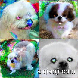
Figure 1: Class-conditional samples generated by our model.
图1:我们的模型生成的类条件样本。
The state of generative image modeling has advanced dramatically in recent years, with Generative Adversarial Networks (GANs, Goodfellow et al. (2014)) at the forefront of efforts to generate high-fidelity, diverse images with models learned directly from data. GAN training is dynamic, and sensitive to nearly every aspect of its setup (from optimization parameters to model architecture), but a torrent of research has yielded empirical and theoretical insights enabling stable training in a variety of settings. Despite this progress, the current state of the art in conditional ImageNet modeling (Zhang et al., 2018) achieves an Inception Score (Salimans et al., 2016) of 52.5, compared to 233 for real data.
近年来,生成图像建模的状态有了显着进步,生成对抗网络(GANs,Goodfellow et al。(2014))致力于通过使用直接从数据中学习的模型来生成高保真,多样化的图像。GAN训练是动态的,并且对设置的几乎每个方面都敏感(从优化参数到模型体系结构),但是大量研究已经获得了经验和理论见解,可以在各种环境中进行稳定的训练。尽管取得了这些进展,但条件ImageNet建模的最新技术(Zhang等人,2018年)仍达到了初始分数(Salimans等人,2016年)。 为52.5,而实际数据为233。
In this work, we set out to close the gap in fidelity and variety between images generated by GANs and real-world images from the ImageNet dataset. We make the following three contributions towards this goal:
在这项工作中,我们着手缩小GAN生成的图像与ImageNet数据集中的真实世界图像之间在保真度和多样性上的差距。我们为实现该目标做出了以下三点贡献:
- We demonstrate that GANs benefit dramatically from scaling, and train models with two to four times as many parameters and eight times the batch size compared to prior art. We introduce two simple, general architectural changes that improve scalability, and modify a regularization scheme to improve conditioning, demonstrably boosting performance.
- As a side effect of our modifications, our models become amenable to the “truncation trick,” a simple sampling technique that allows explicit, fine-grained control of the trade-off between sample variety and fidelity.
- We discover instabilities specific to large scale GANs, and characterize them empirically. Leveraging insights from this analysis, we demonstrate that a combination of novel and existing techniques can reduce these instabilities, but complete training stability can only be achieved at a dramatic cost to performance.
- 我们证明了GAN可以极大地受益于缩放,并且与现有技术相比,可以训练具有两倍至四倍的参数和八倍的批量大小的模型。我们介绍了两个简单的,通用的体系结构更改,这些更改可提高可伸缩性,并修改正则化方案以改善条件,从而明显提高性能。
- 作为我们修改的副作用,我们的模型适合“截断技巧”,这是一种简单的采样技术,可以显式,细粒度地控制样本种类与保真度之间的折衷。
- 我们发现了针对大型GAN的不稳定性,并根据经验对其进行了表征。利用来自此分析的见解,我们证明了将新颖的技术与现有的技术相结合可以减少这些不稳定性,但是要达到完全的训练稳定性,就必须付出巨大的性能代价。
Our modifications substantially improve class-conditional GANs. When trained on ImageNet at 128×128 resolution, our models (BigGANs) improve the state-of-the-art Inception Score (IS) and Fréchet Inception Distance (FID) from 52.52 and 18.65 to 166.3 and 9.6 respectively. We also successfully train BigGANs on ImageNet at 256×256 and 512×512 resolution, and achieve IS and FID of 233.0 and 9.3 at 256×256 and IS and FID of 241.4 and 10.9 at 512×512. Finally, we train our models on an even larger dataset – JFT-300M – and demonstrate that our design choices transfer well from ImageNet.
我们的修改大大改善了类条件GAN。在ImageNet上于128进行培训时×我们的模型(BigGAN)的分辨率为128,将最先进的起始分数(IS)和弗雷谢特起始距离(FID)从52.52和18.65分别提高到166.3和9.6。我们还成功地在256的ImageNet上训练了BigGAN×256和512×512分辨率,并在256时达到233.0和9.3的IS和FID×256,IS和FID为241.4和10.9(512)×512.最后,我们在更大的数据集– JFT-300M上训练模型,并证明我们的设计选择可以很好地从ImageNet转移。
2BACKGROUND
A Generative Adversarial Network (GAN) involves Generator (G) and Discriminator (D) networks whose purpose, respectively, is to map random noise to samples and discriminate real and generated samples. Formally, the GAN objective, in its original form (Goodfellow et al., 2014) involves finding a Nash equilibrium to the following two player min-max problem:
生成对抗网络(GAN)涉及生成器(G)和鉴别器(D)网络,它们的目的分别是将随机噪声映射到样本,并区分真实样本和生成的样本。形式上,GAN目标的正式形式(Goodfellow等,2014)涉及找到以下两个参与者的最小-最大问题的纳什均衡:

$$
\min_{G}\max_{D} E_{x~q_data(x)}[log D(x)]+E_z \sim p(z)}[log(1-D(G(z))) $$
where$z\in\mathbb{R}^{d_z}$ is a latent variable drawn from distribution p(z) such as N(0,I) or U[−1,1]. When applied to images, G and D are usually convolutional neural networks (Radford et al., 2016). Without auxiliary stabilization techniques, this training procedure is notoriously brittle, requiring finely-tuned hyperparameters and architectural choices to work at all.
Much recent research has accordingly focused on modifications to the vanilla GAN procedure to impart stability, drawing on a growing body of empirical and theoretical insights (Nowozin et al., 2016; Sønderby et al., 2017; Fedus et al., 2018). One line of work is focused on changing the objective function (Arjovsky et al., 2017; Mao et al., 2016; Lim & Ye, 2017; Bellemare et al., 2017; Salimans et al., 2018) to encourage convergence. Another line is focused on constraining D through gradient penalties (Gulrajani et al., 2017; Kodali et al., 2017; Mescheder et al., 2018) or normalization (Miyato et al., 2018), both to counteract the use of unbounded loss functions and ensure D provides gradients everywhere to G.
当应用于图像时,G和D通常是卷积神经网络(Radford et al。,2016)。没有辅助稳定技术,该训练过程非常脆弱,需要经过微调的超参数和体系结构选择才能完全起作用。
因此,最近的许多研究都集中在对香草GAN程序的修改上,以赋予稳定性,并利用了越来越多的经验和理论见解(Nowozin等人,2016 ;Sønderby等人,2017 ; Fedus等人,2018)。一项工作重点是改变目标函数(Arjovsky等人,2017 ; Mao等人,2016 ; Lim&Ye,2017 ; Bellemare等人,2017 ; Salimans等人,2018)以鼓励融合。另一条线着重于通过梯度惩罚来约束D (Gulrajani et al。,2017; Kodali等人,2017年;Mescheder et al。,2018)或归一化(Miyato et al。,2018),既可以抵消无界损失函数的使用,又可以确保D到G各处都提供梯度。
Of particular relevance to our work is Spectral Normalization (Miyato et al., 2018), which enforces Lipschitz continuity on D by normalizing its parameters with running estimates of their first singular values, inducing backwards dynamics that adaptively regularize the top singular direction. Relatedly Odena et al. (2018) analyze the condition number of the Jacobian of G and find that performance is dependent on G’s conditioning. Zhang et al. (2018) find that employing Spectral Normalization in G improves stability, allowing for fewer D steps per iteration. We extend on these analyses to gain further insight into the pathology of GAN training.
与我们的工作特别相关的是光谱归一化(Miyato等人,2018年),该方法通过使用其第一个奇异值的运行估计值对其参数进行归一化来归因于D上的Lipschitz连续性,并引入向后动力学以自适应地对顶部奇异方向进行正则化。有关Odena等。(2018)分析G的雅可比行列的条件数,发现性能取决于G的条件。张等。(2018)发现在G中使用频谱归一化可提高稳定性,从而减少D每次迭代的步骤。我们扩展了这些分析,以进一步了解GAN训练的病理学。
Other works focus on the choice of architecture, such as SA-GAN (Zhang et al., 2018) which adds the self-attention block from (Wang et al., 2018) to improve the ability of both G and D to model global structure. ProGAN (Karras et al., 2018) trains high-resolution GANs in the single-class setting by training a single model across a sequence of increasing resolutions.
其他工作着重于架构的选择,例如SA-GAN (Zhang等人,2018年),它增加了(Wang等人,2018年)的自注意力模块,以提高G和D建模全局的能力结构体。ProGAN (Karras et al。,2018)通过在一系列分辨率提高的情况下训练单个模型来在单班环境中训练高分辨率GAN。
In conditional GANs (Mirza & Osindero, 2014) class information can be fed into the model in various ways. In (Odena et al., 2017) it is provided to G by concatenating a 1-hot class vector to the noise vector, and the objective is modified to encourage conditional samples to maximize the corresponding class probability predicted by an auxiliary classifier. de Vries et al. (2017) and Dumoulin et al. (2017) modify the way class conditioning is passed to G by supplying it with class-conditional gains and biases in BatchNorm (Ioffe & Szegedy, 2015) layers. In Miyato & Koyama (2018), D is conditioned by using the cosine similarity between its features and a set of learned class embeddings as additional evidence for distinguishing real and generated samples, effectively encouraging generation of samples whose features match a learned class prototype.
在有条件的GAN中(Mirza和Osindero,2014年),可以通过多种方式将类信息输入模型。在(Odena et al。,2017)中,它通过将1-hot类向量与噪声向量连接而提供给G,并修改了目标以鼓励条件样本最大化由辅助分类器预测的相应类概率。de Vries等。(2017)和Dumoulin等。(2017)修改类条件传递给G的方式,方法是为它提供BatchNorm中的类条件增益和偏差(Ioffe&Szegedy,2015)图层。在Miyato&Koyama(2018)中,D是通过使用其特征和一组学习的类嵌入之间的余弦相似性作为条件来区分D和真实样本和生成的样本的条件,从而有效地鼓励生成其特征与学习的类原型相匹配的样本。
Objectively evaluating implicit generative models is difficult (Theis et al., 2015). A variety of works have proposed heuristics for measuring the sample quality of models without tractable likelihoods (Salimans et al., 2016; Heusel et al., 2017; Bińkowski et al., 2018; Wu et al., 2017). Of these, the Inception Score (IS, Salimans et al. (2016)) and Fréchet Inception Distance (FID, Heusel et al. (2017)) have become popular despite their notable flaws (Barratt & Sharma, 2018). We employ them as approximate measures of sample quality, and to enable comparison against previous work.
客观地评估隐式生成模型是困难的(Theis等,2015)。各种各样的工作提出了启发式方法来测量模型的样本质量而没有难以预测的可能性(Salimans等人,2016 ; Heusel等人,2017 ;Bińkowski等人,2018 ; Wu等人,2017)。其中,Inception Score(IS,Salimans et al。(2016))和FréchetInception Distance(FID,Heusel et al。(2017))尽管存在明显的缺陷(Barratt&Sharma,2018),但它们仍然很受欢迎。。我们将它们用作样本质量的近似度量,并能够与以前的工作进行比较。
3 SCALING UP GANS
| Batch | Ch. | Param (M) | Shared | Hier. | Ortho. | Itr ×103 | FID | IS |
|---|---|---|---|---|---|---|---|---|
| 256 | 64 | 81.5 | SA-GAN Baseline | 1000 | 18.65 | 52.52 | ||
| 512 | 64 | 81.5 | ✗ | ✗ | ✗ | 1000 | 15.30 | 58.77(±1.18) |
| 1024 | 64 | 81.5 | ✗ | ✗ | ✗ | 1000 | 14.88 | 63.03(±1.42) |
| 2048 | 64 | 81.5 | ✗ | ✗ | ✗ | 732 | 12.39 | 76.85(±3.83) |
| 2048 | 96 | 173.5 | ✗ | ✗ | ✗ | 295(±18) | 9.54(±0.62) | 92.98(±4.27) |
| 2048 | 96 | 160.6 | ✓ | ✗ | ✗ | 185(±11) | 9.18(±0.13) | 94.94(±1.32) |
| 2048 | 96 | 158.3 | ✓ | ✓ | ✗ | 152(±7) | 8.73(±0.45) | 98.76(±2.84) |
| 2048 | 96 | 158.3 | ✓ | ✓ | ✓ | 165(±13) | 8.51(±0.32) | 99.31(±2.10) |
| 2048 | 64 | 71.3 | ✓ | ✓ | ✓ | 371(±7) | 10.48(±0.10) | 86.90(±0.61) |
Table 1: Fréchet Inception Distance (FID, lower is better) and Inception Score (IS, higher is better) for ablations of our proposed modifications. Batch is batch size, Param is total number of parameters, Ch. is the channel multiplier representing the number of units in each layer, Shared is using shared embeddings, Hier. is using a hierarchical latent space, Ortho. is Orthogonal Regularization, and Itr either indicates that the setting is stable to 106 iterations, or that it collapses at the given iteration. Other than rows 1-4, results are computed across 8 different random initializations.
表1:我们建议的修改的消融的弗雷谢特起始距离(FID,越低越好)和起始分数(IS,越高越好)。批次是批次大小,参数是参数总数,通道。是表示每个图层中单位数量的渠道乘数,“共享”使用共享嵌入,即“层数”。正在使用分层潜伏空间Ortho。是正交正则化,并且Itr要么表明设置对106迭代,或者它在给定的迭代中崩溃。除了第1-4行,结果是在8种不同的随机初始化中计算得出的。
In this section, we explore methods for scaling up GAN training to reap the performance benefits of larger models and larger batches. As a baseline, we employ the SA-GAN architecture of Zhang et al. (2018), which uses the hinge loss (Lim & Ye, 2017; Tran et al., 2017) GAN objective. We provide class information to G with class-conditional BatchNorm (Dumoulin et al., 2017; de Vries et al., 2017) and to D with projection (Miyato & Koyama, 2018). The optimization settings follow Zhang et al. (2018) (notably employing Spectral Norm in G) with the modification that we halve the learning rates and take two D steps per G step. For evaluation, we employ moving averages of G’s weights following Karras et al. (2018); Mescheder et al. (2018), with a decay of 0.9999. We use Orthogonal Initialization (Saxe et al., 2014), whereas previous works used N(0,0.02I) (Radford et al., 2016) or Xavier initialization (Glorot & Bengio, 2010). Each model is trained on 128 to 512 cores of a Google TPU v3 Pod (Google, 2018), and computes BatchNorm statistics in G across all devices, rather than per-device as in standard implementations. We find progressive growing (Karras et al., 2018) unnecessary even for our largest 512×512 models.
在本节中,我们探索扩大GAN训练规模的方法,以获取更大模型和更大批次的性能收益。作为基准,我们采用了Zhang等人的SA-GAN体系结构。(2018),它使用了铰链损耗(Lim&Ye,2017 ; Tran等,2017) GAN目标。我们提供的等级信息到ģ与分类条件BatchNorm (等人迪穆兰,。2017 ;德Vries等,2017年)和d与突出部(宫户&小山,2018)。优化设置遵循Zhang等人的方法。(2018年)(尤其是在G中使用频谱范数),并进行了修改,使我们将学习率减半,并且每G步采取两个D步。为了进行评估,我们采用了Karras等人的G权重的移动平均值。(2018); Mescheder等。(2018),衰落了。0.9999。我们使用正交初始化(Saxe et al。,2014),而以前的工作使用ñ(0,0.02一世) (Radford等人,2016)或Xavier初始化(Glorot&Bengio,2010)。每种模型都在Google TPU v3 Pod的128至512核上进行了训练 (Google,2018年),并在所有设备上以G形式计算BatchNorm统计信息,而不是像标准实现那样按设备计算。我们发现即使对于我们最大的512家,也无需进行渐进式增长(Karras等人,2018年)×512个型号。
We begin by increasing the batch size for the baseline model, and immediately find tremendous benefits in doing so. Rows 1-4 of Table 1 show that simply increasing the batch size by a factor of 8 improves the state-of-the-art IS by 46%. We conjecture that this is a result of each batch covering more modes, providing better gradients for both networks. One notable side effect of this scaling is that our models reach better final performance in fewer iterations, but become unstable and undergo complete training collapse. We discuss the causes and ramifications of this in Section 4. For these experiments, we stop training just after collapse, and report scores from checkpoints saved just before.
We then increase the width (number of channels) in every layer by 50%, approximately doubling the number of parameters in both models. This leads to a further IS improvement of 21%, which we posit is due to the increased capacity of the model relative to the complexity of the dataset. Doubling the depth does not appear to have the same effect on ImageNet models, instead degrading performance.
我们首先增加基线模型的批次大小,然后立即发现这样做的巨大好处。表1的第1-4行 显示,仅将批次大小增加8倍就可以将最新的IS提升46%。我们推测这是每批覆盖更多模式的结果,从而为两个网络都提供了更好的渐变。这种缩放的一个显着的副作用是我们的模型在较少的迭代中达到了更好的最终性能,但是变得不稳定并经历了完全的训练崩溃。我们将在第4节中讨论此问题的原因和后果 。对于这些实验,我们会在崩溃后立即停止训练,并报告之前保存的检查点的得分。
然后,我们将每层的宽度(通道数)增加50%,这几乎使两个模型中的参数数增加了一倍。这导致IS进一步提高21%,这是由于相对于数据集的复杂性,模型的容量增加了。深度加倍似乎对ImageNet模型没有相同的影响,反而会降低性能。
We note that class embeddings c used for the conditional BatchNorm layers in G contain a large number of weights. Instead of having a separate layer for each embedding (Miyato et al., 2018; Zhang et al., 2018), we opt to use a shared embedding, which is linearly projected to each layer’s gains and biases (Perez et al., 2018). This reduces computation and memory costs, and improves training speed (in number of iterations required to reach a given performance) by 37%. Next, we employ a variant of hierarchical latent spaces, where the noise vector z is fed into multiple layers of G rather than just the initial layer. The intuition behind this design is to allow G to use the latent space to directly influence features at different resolutions and levels of hierarchy. For our architecture, this is easily accomplished by splitting z into one chunk per resolution, and concatenating each chunk to the conditional vector c which gets projected to the BatchNorm gains and biases. Previous works (Goodfellow et al., 2014; Denton et al., 2015) have considered variants of this concept; our contribution is a minor modification of this design. Hierarchical latents improve memory and compute costs (primarily by reducing the parametric budget of the first linear layer), provide a modest performance improvement of around 4%, and improve training speed by a further 18%.
我们注意到类嵌入 C用于G中的条件BatchNorm层的层包含大量权重。我们没有使用每个嵌入单独的层 (Miyato等人,2018 ; Zhang等人,2018),而是选择使用共享嵌入,将其线性投影到每一层的增益和偏差 (Perez等人,2018))。这样可以减少计算和内存成本,并将训练速度(达到给定性能所需的迭代次数)提高37%。接下来,我们使用分层潜伏空间的一种变体,其中噪声矢量ž被送入G的多个层,而不仅仅是初始层。这种设计的直觉是允许G使用潜在空间直接影响处于不同分辨率和层次级别的要素。对于我们的体系结构,这很容易通过拆分来完成ž 每个分辨率分成一个块,然后将每个块连接到条件向量 C可以预测到BatchNorm的增益和偏差。先前的工作(Goodfellow等,2014; Denton等,2015)已经考虑了该概念的变体。我们的贡献是对该设计的微小修改。分层的潜能改善了内存和计算成本(主要是通过减少第一线性层的参数预算),提供了大约4%的适度性能改进,并进一步提高了18%的训练速度。
3.1TRADING OFF VARIETY AND FIDELITY WITH THE TRUNCATION TRICK 在“截断技巧”中权衡多样性和忠诚度
 |
 |
 |
 |
|---|
(a)
(b)
Figure 2: (a) The effects of increasing truncation. From left to right, threshold=2, 1.5, 1, 0.5, 0.04. (b) Saturation artifacts from applying truncation to a poorly conditioned model.Unlike models which need to backpropagate through their latents, GANs can employ an arbitrary prior p(z), yet the vast majority of previous works have chosen to draw z from either N(0,I) or U[−1,1]. We question the optimality of this choice and explore alternatives in Appendix E.
图2:(a)增加截断的影响。从左至右,阈值= 2、1.5、1、0.5、0.04。(b)通过将截断应用于条件较差的模型而产生的饱和伪影。
Remarkably, our best results come from using a different latent distribution for sampling than was used in training. Taking a model trained with z∼N(0,I) and sampling z from a truncated normal (where values which fall outside a range are resampled to fall inside that range) immediately provides a boost to IS and FID. We call this the Truncation Trick: truncating a z vector by resampling the values with magnitude above a chosen threshold leads to improvement in individual sample quality at the cost of reduction in overall sample variety. Figure 2(a) demonstrates this: as the threshold is reduced, and elements of z are truncated towards zero (the mode of the latent distribution), individual samples approach the mode of G’s output distribution.
我们质疑这种选择的最优性,并在附录E中探讨替代方案 。
值得注意的是,我们最好的结果来自于使用与训练中不同的潜在分布进行采样。采取训练有素的模型z∼N(0,I) 和采样 z从截断正常(其中落在外侧的范围的值重采样落在该范围内)立即提供一个升压到IS和FID。我们称其为截断技巧:截断一个ž通过对幅度大于选定阈值的值进行重采样,可以降低单个样本的质量,但会降低总体样本种类。图 2(a)证明了这一点:随着阈值的降低,ž被截断为零(潜在分布的模式),单个样本接近G的输出分布的模式。
This technique allows fine-grained, post-hoc selection of the trade-off between sample quality and variety for a given G. Notably, we can compute FID and IS for a range of thresholds, obtaining the variety-fidelity curve reminiscent of the precision-recall curve (Figure 16). As IS does not penalize lack of variety in class-conditional models, reducing the truncation threshold leads to a direct increase in IS (analogous to precision). FID penalizes lack of variety (analogous to recall) but also rewards precision, so we initially see a moderate improvement in FID, but as truncation approaches zero and variety diminishes, the FID sharply drops. The distribution shift caused by sampling with different latents than those seen in training is problematic for many models. Some of our larger models are not amenable to truncation, producing saturation artifacts (Figure 2(b)) when fed truncated noise. To counteract this, we seek to enforce amenability to truncation by conditioning G to be smooth, so that the full space of z will map to good output samples. For this, we turn to Orthogonal Regularization (Brock et al., 2017), which directly enforces the orthogonality condition:
对于给定的G,该技术允许对样本质量和品种之间的折衷进行细粒度的事后选择。值得注意的是,我们可以针对一定范围的阈值计算FID和IS,从而获得让人联想到精确召回曲线的多样性保真度曲线(图 16)。由于IS不会惩罚类条件模型中的多样性,因此降低截断阈值会导致IS直接增加(类似于精度)。FID会惩罚缺乏多样性的情况(类似于召回),但也会奖励精确度,因此我们最初看到FID有所改善,但随着截断趋近于零且多样性减少,FID急剧下降。对于许多模型来说,由与训练中看到的潜能不同的潜在采样引起的分布偏移是有问题的。我们的某些较大模型不适合截断,在馈入截断噪声时会产生饱和伪像(图 2(b))。为了解决这个问题,我们试图通过将G调整为平滑来增强对截断的适应性,从而使G的整个空间ž将映射到良好的输出样本。为此,我们转向正交正则化(Brock et al。,2017),它直接执行正交条件:
$$
R_{\beta}(W)=\beta|W^{\top}W-I|_{\mathrm{F}}^{2}$$
where W is a weight matrix and β a hyperparameter. This regularization is known to often be too limiting (Miyato et al., 2018), so we explore several variants designed to relax the constraint while still imparting the desired smoothness to our models. The version we find to work best removes the diagonal terms from the regularization, and aims to minimize the pairwise cosine similarity between filters but does not constrain their norm:
W是权重矩阵, β超参数。已知这种正则化通常过于局限(Miyato et al。,2018),因此我们探索了几种旨在放松约束同时仍为模型赋予所需平滑度的变体。我们发现效果最好的版本从正则化中删除了对角项,旨在最大程度地减少滤波器之间的成对余弦相似度,但不限制其范数:
$$
R_{\beta}(W)=\beta|W^{\top}W\odot(\mathbf{1}-I)|_{\mathrm{F}}^{2}$$
where 1 denotes a matrix with all elements set to 1. We sweep β values and select 10−4, finding this small additional regularization sufficient to improve the likelihood that our models will be amenable to truncation. Across runs in Table 1, we observe that without Orthogonal Regularization, only 16% of models are amenable to truncation, compared to 60% when trained with Orthogonal Regularization.
1 表示所有元素均设置为的矩阵 1个。我们遍历β 值并选择 $10^-4$,发现此小的附加正则化足以提高我们的模型可被截断的可能性。在表1的所有运行中 ,我们观察到没有正交正则化的模型只有16%可以被截断,而经过正交正则化训练的模型为60%。
3.2SUMMARY
We find that current GAN techniques are sufficient to enable scaling to large models and distributed, large-batch training. We find that we can dramatically improve the state of the art and train models up to 512×512 resolution without need for explicit multiscale methods like Karras et al. (2018). Despite these improvements, our models undergo training collapse, necessitating early stopping in practice. In the next two sections we investigate why settings which were stable in previous works become unstable when applied at scale.
我们发现,当前的GAN技术足以实现按比例缩放到大型模型和分布式,大批量训练。我们发现我们可以极大地改善现有技术并训练高达512个模型×无需像Karras等人那样的显式多尺度方法即可实现512分辨率。(2018)。尽管有这些改进,但我们的模型仍遭受训练崩溃,因此必须在实践中尽早停止。在接下来的两节中,我们研究了为什么以前的工作中稳定的设置在大规模应用时会变得不稳定。
4 ANALYSIS
 |
 |
|---|---|
| (a) G | (b) D |
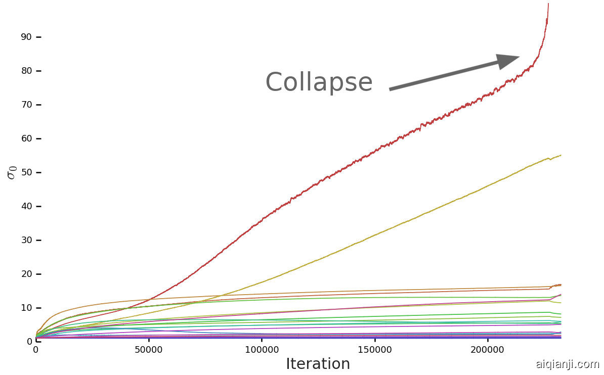
Figure 3: A typical plot of the first singular value σ0 in the layers of G (a) and D (b) before Spectral Normalization. Most layers in G have well-behaved spectra, but without constraints a small subset grow throughout training and explode at collapse. D’s spectra are noisier but otherwise better-behaved. Colors from red to violet indicate increasing depth.
图3:第一个奇异值的典型图σ0在频谱归一化之前的G(a)和D(b)层中。G中的大多数层都具有良好的频谱,但是在没有限制的情况下,一小部分子集会在整个训练过程中增长并在坍塌时爆炸。D的频谱噪声较大,但在其他方面却表现得更好。从红色到紫色的颜色表示深度增加。
4.1CHARACTERIZING INSTABILITY: THE GENERATOR
Much previous work has investigated GAN stability from a variety of analytical angles and on toy problems, but the instabilities we observe occur for settings which are stable at small scale, necessitating direct analysis at large scale. We monitor a range of weight, gradient, and loss statistics during training, in search of a metric which might presage the onset of training collapse, similar to (Odena et al., 2018). We found the top three singular values σ0,σ1,σ2 of each weight matrix to be the most informative. They can be efficiently computed using the Alrnoldi iteration method (Golub & der Vorst, 2000), which extends the power iteration method, used in Miyato et al. (2018), to estimation of additional singular vectors and values. A clear pattern emerges, as can be seen in Figure 3(a) and Appendix F: most G layers have well-behaved spectral norms, but some layers (typically the first layer in G, which is over-complete and not convolutional) are ill-behaved, with spectral norms that grow throughout training and explode at collapse.
以前的许多工作已经从各种分析角度和玩具问题研究了GAN的稳定性,但是我们观察到的不稳定情况发生在小规模稳定的情况下,因此需要大规模直接分析。我们在训练过程中监视一系列重量,梯度和损失统计数据,以寻找可能预示训练崩溃开始的指标,类似于(Odena et al。,2018)。我们找到了前三个奇异值 σ0,σ1个,σ2个每个权重矩阵中的,以提供最多的信息。可以使用Alrnoldi迭代方法(Golub&der Vorst,2000)有效地计算它们 ,该方法扩展了Miyato等人中使用的幂迭代方法 。(2018),以估计其他奇异向量和值。如图3(a)和附录 F所示,出现了清晰的模式 :大多数G层具有良好的频谱范数,但有些层(通常是G中的第一层是过度完成的而不是卷积的)表现不佳,频谱规范会在整个训练过程中不断增长,并在崩溃时爆炸。
To ascertain if this pathology is a cause of collapse or merely a symptom, we study the effects of imposing additional conditioning on G to explicitly counteract spectral explosion. First, we directly regularize the top singular values σ0 of each weight, either towards a fixed value σreg or towards some ratio r of the second singular value, r⋅sg(σ1) (with sg the stop-gradient operation to prevent the regularization from increasing σ1). Alternatively, we employ a partial singular value decomposition to instead clamp σ0. Given a weight W, its first singular vectors u0 and v0, and σclamp the value to which the σ0 will be clamped, our weights become:
为了确定这种病理是崩溃的原因还是仅仅是症状,我们研究了在G上施加额外条件以明显抵消光谱爆炸的影响。首先,我们直接对顶部奇异值进行正则化σ0 每个重量的一个,或者朝着固定值的方向移动
$$
W=W-\max(0,\sigma_{0}-\sigma_{clamp})v_{0}u_{0}^{\top}
$$
where σclamp is set to either σreg or r⋅sg(σ1). We observe that both with and without Spectral Normalization these techniques have the effect of preventing the gradual increase and explosion of either σ0 or σ0σ1, but even though in some cases they mildly improve performance, no combination prevents training collapse. This evidence suggests that while conditioning G might improve stability, it is insufficient to ensure stability. We accordingly turn our attention to D.
4.2CHARACTERIZING INSTABILITY: THE DISCRIMINATOR
As with G, we analyze the spectra of D’s weights to gain insight into its behavior, then seek to stabilize training by imposing additional constraints. Figure 3(b) displays a typical plot of σ0 for D (with further plots in Appendix F). Unlike G, we see that the spectra are noisy, σ0σ1 is well-behaved, and the singular values grow throughout training but only jump at collapse, instead of exploding.
The spikes in D’s spectra might suggest that it periodically receives very large gradients, but we observe that the Frobenius norms are smooth (Appendix F), suggesting that this effect is primarily concentrated on the top few singular directions. We posit that this noise is a result of optimization through the adversarial training process, where G periodically produces batches which strongly perturb D . If this spectral noise is causally related to instability, a natural counter is to employ gradient penalties, which explicitly regularize changes in D’s Jacobian. We explore the R1 zero-centered gradient penalty from Mescheder et al. (2018):
D光谱的尖峰可能表明它周期性地接收到很大的梯度,但是我们观察到Frobenius范数是平滑的(附录 F),这表明该效应主要集中在前几个奇异方向上。我们认为,这种噪声是通过对抗训练过程进行优化的结果,其中G周期性地产生强烈干扰D的批次。如果此频谱噪声与不稳定性有因果关系,则自然的对策是采用梯度罚分法,该罚分法明确地规范了D氏雅可比定律的变化。我们探索[R1个Mescheder等人的零中心梯度惩罚。(2018):
$$
R_{1}:=\frac{\gamma}{2}\E_{p_D(x)}[|\nabla D(x)|_{F%
}^{2}]
$$
With the default suggested γ strength of 10, training becomes stable and improves the smoothness and boundedness of spectra in both G and D, but performance severely degrades, resulting in a 45% reduction in IS. Reducing the penalty partially alleviates this degradation, but results in increasingly ill-behaved spectra; even with the penalty strength reduced to 1 (the lowest strength for which sudden collapse does not occur) the IS is reduced by 20%. Repeating this experiment with various strengths of Orthogonal Regularization, DropOut (Srivastava et al., 2014), and L2 (See Appendix H for details), reveals similar behaviors for these regularization strategies: with high enough penalties on D, training stability can be achieved, but at a substantial cost to performance.
默认情况下建议 γ强度为10时,训练变得稳定并改善了G和D光谱的平滑度和有界性,但是性能严重下降,导致IS降低了45%。减少损失可以部分缓解这种退化,但会导致不良行为光谱的增加;即使惩罚强度降低到1个(不会发生突然崩溃的最低强度)IS降低了20%。用正交正则化,DropOut (Srivastava等人,2014)和L2(请参见附录 H的详细信息)的各种强度重复该实验,发现这些正则化策略具有相似的行为:对D施加足够高的惩罚,可以实现训练稳定性,但会大幅降低性能。
We also observe that D’s loss approaches zero during training, but undergoes a sharp upward jump at collapse (Appendix F). One possible explanation for this behavior is that D is overfitting to the training set, memorizing training examples rather than learning some meaningful boundary between real and generated images. As a simple test for D’s memorization (related to Gulrajani et al. (2017)), we evaluate uncollapsed discriminators on the ImageNet training and validation sets, and measure what percentage of samples are classified as real or generated. While the training accuracy is consistently above 98%, the validation accuracy falls in the range of 50-55%, no better than random guessing (regardless of regularization strategy). This confirms that D is indeed memorizing the training set; we deem this in line with D’s role, which is not explicitly to generalize, but to distill the training data and provide a useful learning signal for G.
我们还观察到D的损失在训练过程中接近零,但在崩溃时会急剧上升(附录 F)。对此行为的一种可能解释是,D过度适合训练集,记住训练示例,而不是学习真实图像与生成图像之间的有意义边界。作为D记忆的简单测试(与Gulrajani等人(2017年)有关)),我们在ImageNet训练和验证集上评估未折叠的鉴别器,并测量将样本分类为真实样本还是生成样本的百分比。尽管训练准确性始终高于98%,但验证准确性却落在50-55%的范围内,没有比随机猜测更好的了(不管正则化策略如何)。这证实了D 确实在记住训练集。我们认为这与D的作用相符,D的作用不是明确概括,而是提取训练数据并为G提供有用的学习信号。
4.3SUMMARY
We find that stability does not come solely from G or D, but from their interaction through the adversarial training process. While the symptoms of their poor conditioning can be used to track and identify instability, ensuring reasonable conditioning proves necessary for training but insufficient to prevent eventual training collapse. It is possible to enforce stability by strongly constraining D, but doing so incurs a dramatic cost in performance. With current techniques, better final performance can be achieved by relaxing this conditioning and allowing collapse to occur at the later stages of training, by which time a model is sufficiently trained to achieve good results.
我们发现稳定性并非仅来自于G或D,而是来自它们在对抗训练过程中的相互作用。虽然他们的不良训练条件的症状可以用来追踪和识别不稳定性,但是确保合理的训练条件被证明是训练所必需的,但不足以防止最终训练失败。可以通过强力约束D来增强稳定性,但这样做会导致巨大的性能损失。使用当前的技术,可以通过放松此条件并允许在训练的后续阶段发生崩溃来获得更好的最终性能,这时将对模型进行充分的训练以达到良好的效果。
5EXPERIMENTS
| |  |
|
| - |
| (a) 128×128 |
| |  |
|
| - |
| (b) 256×256 |
| |  |
|
| - |
| (c) 512×512 |
| |  |
|
| - |
| (d) |
Figure 4: Samples from our model with truncation threshold 0.5 (a-c) and an example of class leakage in a partially trained model (d).| Model | Res. | FID/IS | (min FID) / IS | FID / (valid IS) | FID / (max IS) |
| - | - | - | - | - | - |
|
SN-GAN | 128 | 27.62 / 36.80 | N/A | N/A | N/A |
|
SA-GAN | 128 | 18.65 / 52.52 | N/A | N/A | N/A |
|
BigGAN | 128 | 8.7±.6/98.8±2.8 | 7.7±.1/126.5±.1 | 9.6±.4/166.3±1 | 25±2/206±2 |
|
BigGAN | 256 | 8.2±.2/154±2.5 | 7.7±.1/178±5 | 9.3±.3/233±1 | 25±5/295±4 |
|
BigGAN | 512 | 10.9 / 154.9 | 9.3 / 202.5 | 10.9 / 241.4 | 24.4/275 |
|
| | | | | |
Table 2: Evaluation of models at different resolutions. We report scores without truncation (Column 3), scores at the best FID (Column 4), scores at the IS of validation data (Column 5), and scores at the max IS (Column 6). Standard deviations are computed over at least three random initializations.### 5.1EVALUATION ON IMAGENET
We evaluate our models on ImageNet ILSVRC 2012 (Russakovsky et al., 2015) at 128×128, 256×256, and 512×512 resolutions, employing the settings from Table 1, row 8. Architectural details for each resolution are available in Appendix B. Samples are presented in Figure 4, with additional samples in Appendix A, and we report IS and FID in Table 2. As our models are able to trade sample variety for quality, it is unclear how best to compare against prior art; we accordingly report values at three settings, with detailed curves in Appendix D. First, we report the FID/IS values at the truncation setting which attains the best FID. Second, we report the FID at the truncation setting for which our model’s IS is the same as that attained by the real validation data, reasoning that this is a passable measure of maximum sample variety achieved while still achieving a good level of “objectness.” Third, we report FID at the maximum IS achieved by each model, to demonstrate how much variety must be traded off to maximize quality. In all three cases, our models outperform the previous state-of-the-art IS and FID scores achieved by Miyato et al. (2018) and Zhang et al. (2018).
Our observation that D overfits to the training set, coupled with our model’s sample quality, raises the obvious question of whether or not G simply memorizes training points. To test this, we perform class-wise nearest neighbors analysis in pixel space and the feature space of pre-trained classifier networks (Appendix A). In addition, we present both interpolations between samples and class-wise interpolations (where z is held constant) in Figures 8 and 9. Our model convincingly interpolates between disparate samples, and the nearest neighbors for its samples are visually distinct, suggesting that our model does not simply memorize training data.
We note that some failure modes of our partially-trained models are distinct from those previously observed. Most previous failures involve local artifacts (Odena et al., 2016), images consisting of texture blobs instead of objects (Salimans et al., 2016), or the canonical mode collapse. We observe class leakage, where images from one class contain properties of another, as exemplified by Figure 4(d). We also find that many classes on ImageNet are more difficult than others for our model; our model is more successful at generating dogs (which make up a large portion of the dataset, and are mostly distinguished by their texture) than crowds (which comprise a small portion of the dataset and have more large-scale structure). Further discussion is available in Appendix A.
我们在128的ImageNet ILSVRC 2012 (Russakovsky et al。,2015)上评估了我们的模型 ×128、256×256和512×512种分辨率,采用表1第8行中的设置 。每种分辨率的体系结构详细信息在附录 B中提供。图4中显示了 示例,附录A中提供了其他示例 ,我们在表2中报告了IS和FID 。由于我们的模型能够以质量为代价交换样本品种,因此尚不清楚如何最好地与现有技术进行比较。因此,我们报告了三种设置的值,附录D中有详细的曲线 。首先,我们在达到最佳FID的截断设置下报告FID / IS值。其次,我们在截断设置下报告FID,该截断设置下我们模型的IS与真实验证数据所获得的FIS相同,理由是这是在达到良好“客观性”水平的前提下可以实现的最大样本多样性的衡量标准。第三,我们报告每个模型达到的最大IS的FID,以说明必须权衡多少品种才能最大化质量。在所有这三种情况下,我们的模型均优于Miyato等人先前获得的最新的IS和FID评分。(2018)和Zhang等。(2018)。
我们观察到D过度适合训练集,再加上我们模型的样本质量,提出了一个明显的问题,即G是否仅存储训练点。为了测试这一点,我们在像素空间和预训练分类器网络的特征空间中执行了逐级最近邻分析(附录 A)。此外,我们同时介绍了样本之间的插值和类插值(其中ž在图8和9中保持恒定) 。我们的模型令人信服地在不同样本之间进行插值,并且其样本的最近邻居在视觉上是截然不同的,这表明我们的模型并非简单地记住训练数据。
我们注意到,我们部分训练的模型的某些故障模式与先前观察到的模式不同。先前的大多数故障都涉及局部伪影(Odena等,2016),由纹理斑点而不是对象组成的图像(Salimans等,2016)或规范模式崩溃。我们观察到类泄漏,其中来自一类的图像包含另一类的属性,如图4所示。 (d)。我们还发现,对于我们的模型,ImageNet上的许多类比其他类更难。我们的模型在生成狗(占数据集很大一部分,并且主要由它们的纹理区分)方面比在人群(占数据集的很小一部分并且具有更大的结构)方面更成功。附录A中提供了进一步的讨论 。
5.2ADDITIONAL EVALUATION ON JFT-300M
To confirm that our design choices are effective for even larger and more complex and diverse datasets, we also present results of our system on a subset of JFT-300M (Sun et al., 2017). The full JFT-300M dataset contains 300M real-world images labeled with 18K categories. Since the category distribution is heavily long-tailed, we subsample the dataset to keep only images with the 8.5K most common labels. The resulting dataset contains 292M images – two orders of magnitude larger than ImageNet. For images with multiple labels, we sample a single label randomly and independently whenever an image is sampled. To compute IS and FID for the GANs trained on this dataset, we use an Inception v2 classifier (Szegedy et al., 2016) trained on this dataset. Quantitative results are presented in Table 3. All models are trained with batch size 2048. We compare an ablated version of our model – comparable to SA-GAN (Zhang et al., 2018) but with the larger batch size – against a “full” version that makes uses of all of the techniques applied to obtain the best results on ImageNet (shared embedding, hierarchical latents, and orthogonal regularization). Our results show that these techniques substantially improve performance even in the setting of this much larger dataset at the same model capacity (64 base channels). We further show that for a dataset of this scale, we see significant additional improvements from expanding the capacity of our models to 128 base channels, while for ImageNet GANs that additional capacity was not beneficial.
In Figure 18 (Appendix D), we present truncation plots for models trained on this dataset. Unlike for ImageNet, where truncation limits of σ≈0 tend to produce the highest fidelity scores, IS is typically maximized for our JFT-300M models when the truncation value σ ranges from 0.5 to 1. We suspect that this is at least partially due to the intra-class variability of JFT-300M labels, as well as the relative complexity of the image distribution, which includes images with multiple objects at a variety of scales. Interestingly, unlike models trained on ImageNet, where training tends to collapse without heavy regularization (Section 4), the models trained on JFT-300M remain stable over many hundreds of thousands of iterations. This suggests that moving beyond ImageNet to larger datasets may partially alleviate GAN stability issues.
The improvement over the baseline GAN model that we achieve on this dataset without changes to the underlying models or training and regularization techniques (beyond expanded capacity) demonstrates that our findings extend from ImageNet to datasets with scale and complexity thus far unprecedented for generative models of images.
为了确认我们的设计选择对更大,更复杂和多样化的数据集有效,我们还在JFT-300M的子集上展示了系统结果 (Sun等,2017年)。完整的JFT-300M数据集包含标有18K类别的3亿张真实世界图像。由于类别分布是长尾的,因此我们对数据集进行二次采样,以仅保留带有8.5K最常见标签的图像。结果数据集包含292M图像-比ImageNet大两个数量级。对于带有多个标签的图像,无论何时对图像进行采样,我们都会随机且独立地对单个标签进行采样。为了计算在该数据集上训练的GAN的IS和FID,我们使用了Inception v2分类器 (Szegedy et al。,2016)对此数据集进行了培训。定量结果示于表 3。所有模型都以2048的批次大小进行训练。我们比较了模型的烧蚀版本–与SA-GAN相当 (Zhang等人,2018年)但是批量较大-相对于“完整”版本,该版本利用了所有在ImageNet上获得最佳效果的技术(共享嵌入,分层潜伏和正交正则化)。我们的结果表明,即使在相同的模型容量(64个基本通道)下设置更大的数据集的情况下,这些技术也可以显着提高性能。我们进一步表明,对于这种规模的数据集,我们看到了将模型的容量扩展到128个基本通道的显着其他改进,而对于ImageNet GAN,额外的容量却无济于事。
在图 18(附录 D)中,我们给出了在该数据集上训练的模型的截断图。与ImageNet不同,ImageNet的截断限制为σ≈0 往往会产生最高的保真度得分,当截断值达到最大值时,对于我们的JFT-300M模型,IS通常会最大化 σ范围从0.5到1。我们怀疑这至少部分是由于JFT-300M标签的类内可变性以及图像分布的相对复杂性所致,其中包括具有多个比例的多个对象的图像。有趣的是,与在ImageNet上训练的模型不同,在训练过程中训练趋于崩溃而没有大量的正则化(第4节 ),在JFT-300M上训练的模型在数十万次迭代中保持稳定。这表明,从ImageNet转移到更大的数据集可能会部分缓解GAN稳定性问题。
对我们在该数据集上实现的基线GAN模型的改进没有改变基础模型或训练和正则化技术(超出了扩展能力),表明我们的发现已从ImageNet扩展到具有规模和复杂性的数据集,这对于图像生成模型来说是前所未有的。
| Ch. | Param (M) | Shared | Hier. | Ortho. | FID | IS | (min FID) / IS | FID / (max IS) |
|---|---|---|---|---|---|---|---|---|
| 64 | 317.1 | ✗ | ✗ | ✗ | 48.38 | 23.27 | 48.6 / 23.1 | 49.1 / 23.9 |
| 64 | 99.4 | ✓ | ✓ | ✓ | 23.48 | 24.78 | 22.4 / 21.0 | 60.9 / 35.8 |
| 96 | 207.9 | ✓ | ✓ | ✓ | 18.84 | 27.86 | 17.1 / 23.3 | 51.6 / 38.1 |
| 128 | 355.7 | ✓ | ✓ | ✓ | 13.75 | 30.61 | 13.0 / 28.0 | 46.2 / 47.8 |
Table 3: Results on JFT-300M at 256×256 resolution. The FID and IS columns report these scores given by the JFT-300M-trained Inception v2 classifier with noise distributed as z∼N(0,I) (non-truncated). The (min FID) / IS and FID / (max IS) columns report scores at the best FID and IS from a sweep across truncated noise distributions ranging from σ=0 to σ=2. Images from the JFT-300M validation set have an IS of 50.88 and FID of 1.94.
6CONCLUSION
We have demonstrated that Generative Adversarial Networks trained to model natural images of multiple categories highly benefit from scaling up, both in terms of fidelity and variety of the generated samples. As a result, our models set a new level of performance among ImageNet GAN models, improving on the state of the art by a large margin. We have also presented an analysis of the training behavior of large scale GANs, characterized their stability in terms of the singular values of their weights, and discussed the interplay between stability and performance.
我们已经证明,受过训练的可模拟多种类别自然图像的生殖对抗网络在保真度和生成样本的多样性方面都受益于按比例放大。结果,我们的模型在ImageNet GAN模型中设置了新的性能水平,大大改善了现有技术水平。我们还对大型GAN的训练行为进行了分析,通过权重的奇异值描述了它们的稳定性,并讨论了稳定性和性能之间的相互作用。
Acknowledgments
We would like to thank Kai Arulkumaran, Matthias Bauer, Peter Buchlovsky, Jeffrey Defauw, Sander Dieleman, Ian Goodfellow, Ariel Gordon, Karol Gregor, Dominik Grewe, Chris Jones, Jacob Menick, Augustus Odena, Suman Ravuri, Ali Razavi, Mihaela Rosca, and Jeff Stanway.
REFERENCES
- Abadi et al. (2016) Martín Abadi, Paul Barham, Jianmin Chen, Zhifeng Chen, Andy Davis, Jeffrey Dean, Matthieu Devin, Sanjay Ghemawat, Geoffrey Irving, Michael Isard, Manjunath Kudlur, Josh Levenberg, Rajat Monga, Sherry Moore, Derek Murray, Benoit Steiner, Paul Tucker, Vijay Vasudevan, Pete Warden, Martin Wicke, Yuan Yu, and Xiaoqiang Zheng. TensorFlow: A system for large-scale machine learning. In Proceedings of the 12th USENIX Conference on Operating Systems Design and Implementation, OSDI’16, pp. 265–283, Berkeley, CA, USA, 2016. USENIX Association. ISBN 978-1-931971-33-1. URL http://dl.acm.org/citation.cfm?id=3026877.3026899.
- Arjovsky et al. (2017) Martin Arjovsky, Soumith Chintala, and Léon Bottou. Wasserstein generative adversarial networks. In ICML, 2017.
- Barratt & Sharma (2018) Shane Barratt and Rishi Sharma. A note on the Inception Score. In arXiv preprint arXiv:1801.01973, 2018.
- Bellemare et al. (2017) Marc G. Bellemare, Ivo Danihelka, Will Dabney, Shakir Mohamed, Balaji Lakshminarayanan, Stephan Hoyer, and Rémi Munos. The Cramer distance as a solution to biased Wasserstein gradients. In arXiv preprint arXiv:1705.10743, 2017.
- Bińkowski et al. (2018) Mikolaj Bińkowski, Dougal J. Sutherland, Michael Arbel, and Arthur Gretton. Demystifying MMD GANs. In ICLR, 2018.
- Brock et al. (2017) Andrew Brock, Theodore Lim, J.M. Ritchie, and Nick Weston. Neural photo editing with introspective adversarial networks. In ICLR, 2017.
- Chen et al. (2016) Xi Chen, Yan Duan, Rein Houthooft, John Schulman, Ilya Sutskever, and Pieter Abbeel. Infogan: Interpretable representation learning by information maximizing generative adversarial nets. In NIPS, 2016.
- de Vries et al. (2017) Harm de Vries, Florian Strub, Jérémie Mary, Hugo Larochelle, Olivier Pietquin, and Aaron Courville. Modulating early visual processing by language. In NIPS, 2017.
- Denton et al. (2015) Emily Denton, Soumith Chintala, Arthur Szlam, and Rob Fergus. Deep generative image models using a laplacian pyramid of adversarial networks. In NIPS, 2015.
- Dumoulin et al. (2017) Vincent Dumoulin, Jonathon Shlens, and Manjunath Kudlur. A learned representation for artistic style. In ICLR, 2017.
- Fedus et al. (2018) William Fedus, Mihaela Rosca, Balaji Lakshminarayanan, Andrew M. Dai, Shakir Mohamed, and Ian Goodfellow. Many paths to equilibrium: GANs do not need to decrease a divergence at every step. In ICLR, 2018.
- Glorot & Bengio (2010) Xavier Glorot and Yoshua Bengio. Understanding the difficulty of training deep feedforward neural networks. In AISTATS, 2010.
- Golub & der Vorst (2000) Gene Golub and Henk Van der Vorst. Eigenvalue computation in the 20th century. Journal of Computational and Applied Mathematics, 123:35–65, 2000.
- Goodfellow et al. (2014) Ian Goodfellow, Jean Pouget-Abadie, Mehdi Mirza, Bing Xu, David Warde-Farley, Sherjil Ozair, and Aaron Courville Yoshua Bengio. Generative adversarial nets. In NIPS, 2014.
- Google (2018) Google. Cloud TPUs. https://cloud.google.com/tpu/, 2018.
- Gulrajani et al. (2017) Ishaan Gulrajani, Faruk Ahmed, Martín Arjovsky, Vincent Dumoulin, and Aaron C. Courville. Improved training of Wasserstein GANs. In NIPS, 2017.
- He et al. (2016) Kaiming He, Xiangyu Zhang, Shaoqing Ren, and Jian Sun. Deep residual learning for image recognition. In CVPR, 2016.
- Heusel et al. (2017) Martin Heusel, Hubert Ramsauer, Thomas Unterthiner, Bernhard Nessler, Günter Klambauer, and Sepp Hochreiter. GANs trained by a two time-scale update rule converge to a local nash equilibrium. In NIPS, 2017.
- Ioffe & Szegedy (2015) Sergey Ioffe and Christian Szegedy. Batch normalization: Accelerating deep network training by reducing internal covariate shift. In ICML, 2015.
- Karras et al. (2018) Tero Karras, Timo Aila, Samuli Laine, and Jaakko Lehtinen. Progressive growing of GANs for improved quality, stability, and variation. In ICLR, 2018.
- Kingma & Ba (2014) Diederik Kingma and Jimmy Ba. Adam: A method for stochastic optimization. In ICLR, 2014.
- Kodali et al. (2017) Naveen Kodali, Jacob Abernethy, James Hays, and Zsolt Kira. On convergence and stability of GANs. In arXiv preprint arXiv:1705.07215, 2017.
- Krizhevsky & Hinton (2009) Alex Krizhevsky and Geoffrey Hinton. Learning multiple layers of features from tiny images. 2009.
- Lim & Ye (2017) Jae Hyun Lim and Jong Chul Ye. Geometric GAN. In arXiv preprint arXiv:1705.02894, 2017.
- Mao et al. (2016) Xudong Mao, Qing Li, Haoran Xie, Raymond Y. K. Lau, and Zhen Wang. Least squares generative adversarial networks. In arXiv preprint arXiv:1611.04076, 2016.
- Mescheder et al. (2018) Lars Mescheder, Andreas Geiger, and Sebastian Nowozin. Which training methods for GANs do actually converge? In ICML, 2018.
- Mirza & Osindero (2014) Mehdi Mirza and Simon Osindero. Conditional generative adversarial nets. In arXiv preprint arXiv:1411.1784, 2014.
- Miyato & Koyama (2018) Takeru Miyato and Masanori Koyama. cGANs with projection discriminator. In ICLR, 2018.
- Miyato et al. (2018) Takeru Miyato, Toshiki Kataoka, Masanori Koyama, and Yuichi Yoshida. Spectral normalization for generative adversarial networks. In ICLR, 2018.
- Nowozin et al. (2016) Sebastian Nowozin, Botond Cseke, and Ryota Tomioka. f-GAN: Training generative neural samplers using variational divergence minimization. In NIPS, 2016.
- Odena et al. (2016) Augustus Odena, Vincent Dumoulin, and Chris Olah. Deconvolution and checkerboard artifacts. Distill, 2016. doi: 10.23915/distill.00003. URL http://distill.pub/2016/deconv-checkerboard.
- Odena et al. (2017) Augustus Odena, Christopher Olah, and Jonathon Shlens. Conditional image synthesis with auxiliary classifier GANs. In ICML, 2017.
- Odena et al. (2018) Augustus Odena, Jacob Buckman, Catherine Olsson, Tom B. Brown, Christopher Olah, Colin Raffel, and Ian Goodfellow. Is generator conditioning causally related to GAN performance? In ICML, 2018.
- Perez et al. (2018) Ethan Perez, Florian Strub, Harm de Vries, Vincent Dumoulin, and Aaron Courville. FiLM: Visual reasoning with a general conditioning layer. In AAAI, 2018.
- Radford et al. (2016) Alec Radford, Luke Metz, and Soumith Chintala. Unsupervised representation learning with deep convolutional generative adversarial networks. In ICLR, 2016.
- Russakovsky et al. (2015) Olga Russakovsky, Jia Deng, Hao Su, Jonathan Krause, Sanjeev Satheesh, Sean Ma, Zhiheng Huang, Andrej Karpathy, Aditya Khosla, and Michael Bernstein. ImageNet large scale visual recognition challenge. IJCV, 115:211–252, 2015.
- Salimans & Kingma (2016) Tim Salimans and Diederik Kingma. Weight normalization: A simple reparameterization to accelerate training of deep neural networks. In NIPS, 2016.
- Salimans et al. (2016) Tim Salimans, Ian Goodfellow, Wojciech Zaremba, Vicki Cheung, Alec Radford, and Xi Chen. Improved techniques for training GANs. In NIPS, 2016.
- Salimans et al. (2018) Tim Salimans, Han Zhang, Alec Radford, and Dimitris Metaxas. Improving GANs using optimal transport. In ICLR, 2018.
- Saxe et al. (2014) Andrew Saxe, James McClelland, and Surya Ganguli. Exact solutions to the nonlinear dynamics of learning in deep linear neural networks. In ICLR, 2014.
- Simonyan & Zisserman (2015) Karen Simonyan and Andrew Zisserman. Very deep convolutional networks for large-scale image recognition. In ICLR, 2015.
- Sønderby et al. (2017) Casper Kaae Sønderby, Jose Caballero, Lucas Theis, Wenzhe Shi, and Ferenc Huszár. Amortised map inference for image super-resolution. In ICLR, 2017.
- Srivastava et al. (2014) Nitish Srivastava, Geoffrey Hinton, Alex Krizhevsky, Ilya Sutskever, and Ruslan Salakhutdinov. Dropout: A simple way to prevent neural networks from overfitting. JMLR, 15:1929–1958, 2014.
- Sun et al. (2017) Chen Sun, Abhinav Shrivastava, Saurabh Singh, and Abhinav Gupta. Revisiting unreasonable effectiveness of data in deep learning era. In ICCV, pp. 843–852, 2017.
- Szegedy et al. (2016) Christian Szegedy, Vincent Vanhoucke, Sergey Ioffe, Jonathon Shlens, and Zbigniew Wojna. Rethinking the inception architecture for computer vision. In CVPR, pp. 2818–2826, 2016.
- Theis et al. (2015) Lucas Theis, Aäron van den Oord, and Matthias Bethge. A note on the evaluation of generative models. In arXiv preprint arXiv:1511.01844, 2015.
- Tran et al. (2017) Dustin Tran, Rajesh Ranganath, and David M. Blei. Hierarchical implicit models and likelihood-free variational inference. In NIPS, 2017.
- Wang et al. (2018) Xiaolong Wang, Ross B. Girshick, Abhinav Gupta, and Kaiming He. Non-local neural networks. In CVPR, 2018.
- Wu et al. (2017) Yuhuai Wu, Yuri Burda, Ruslan Salakhutdinov, and Roger B. Grosse. On the quantitative analysis of decoder-based generative models. In ICLR, 2017.
- Zhang et al. (2018) Han Zhang, Ian Goodfellow, Dimitris Metaxas, and Augustus Odena. Self-attention generative adversarial networks. In arXiv preprint arXiv:1805.08318, 2018.