ShuffleNet V2: Practical Guidelines for Efficient CNN Architecture Design
Ningning Ma Xiangyu Zhang Hai-Tao Zheng Jian SunEqual contribution.1 1 Megvii Inc (Face++) 2 Tsinghua University
22 ⋆1 ⋆1221 1 Megvii Inc (Face++) 2 Tsinghua University
ABSTRACT
Currently, the neural network architecture design is mostly guided by the indirect metric of computation complexity, i.e., FLOPs. However, the direct metric, e.g., speed, also depends on the other factors such as memory access cost and platform characterics. Thus, this work proposes to evaluate the direct metric on the target platform, beyond only considering FLOPs. Based on a series of controlled experiments, this work derives several practical guidelines for efficient network design. Accordingly, a new architecture is presented, called ShuffleNet V2. Comprehensive ablation experiments verify that our model is the state-of-the-art in terms of speed and accuracy tradeoff.
当前,神经网络体系结构设计主要由计算复杂度的间接度量即FLOP指导。但是,直接指标(例如速度)也取决于其他因素,例如内存访问成本和平台特性。因此,这项工作建议评估目标平台上的直接指标,而不仅仅是考虑FLOP。在一系列受控实验的基础上,这项工作得出了一些有效的网络设计实用指南。因此,提出了一种称为ShuffleNet V2的新体系结构。全面的消融实验证明,我们的模型在速度和精度的权衡方面是最先进的。
Keywords:
CNN architecture design, efficiency, practical
1INTRODUCTION
The architecture of deep convolutional neutral networks (CNNs) has evolved for years, becoming more accurate and faster. Since the milestone work of AlexNet [1], the ImageNet classification accuracy has been significantly improved by novel structures, including VGG [2], GoogLeNet [3], ResNet [4, 5], DenseNet [6], ResNeXt [7], SE-Net [8], and automatic neutral architecture search [9, 10, 11], to name a few.
深度卷积神经网络(CNN)的架构已发展多年,变得更加准确和快速。由于AlexNet的里程碑工作 [ 1 ]中,ImageNet分类精度已经显著通过新颖结构,包括VGG提高 [ 2 ],GoogLeNet [ 3 ],RESNET [ 4,5 ],DenseNet [ 6 ],ResNeXt [ 7 ], SE-Net的 [ 8 ],以及自动中性架构搜索 [ 9,10,11 ],仅举几例。
Besides accuracy, computation complexity is another important consideration. Real world tasks often aim at obtaining best accuracy under a limited computational budget, given by target platform (e.g., hardware) and application scenarios (e.g., auto driving requires low latency). This motivates a series of works towards light-weight architecture design and better speed-accuracy tradeoff, including Xception [12], MobileNet [13], MobileNet V2 [14], ShuffleNet [15], and CondenseNet [16], to name a few. Group convolution and depth-wise convolution are crucial in these works.
除了准确性之外,计算复杂性是另一个重要的考虑因素。现实世界中的任务通常旨在在有限的计算预算下获得最佳精度,这由目标平台(例如,硬件)和应用场景(例如,自动驾驶需要低延迟)给出。这激发了一系列朝着轻量级架构设计和更好的速度准确性权衡的工作,其中包括Xception [ 12 ],MobileNet [ 13 ],MobileNet V2 [ 14 ],ShuffleNet [ 15 ]和CondenseNet [ 16 ]。很少。在这些工作中,分组卷积和深度卷积至关重要。
To measure the computation complexity, a widely used metric is the number of float-point operations, or FLOPs11In this paper, the definition of FLOPs follows [15], i.e. the number of multiply-adds.. However, FLOPs is an indirect metric. It is an approximation of, but usually not equivalent to the direct metric that we really care about, such as speed or latency. Such discrepancy has been noticed in previous works [17, 18, 14, 19]. For example, MobileNet v2 [14] is much faster than NASNET-A [9] but they have comparable FLOPs. This phenomenon is further exmplified in Figure 1(c)(d), which show that networks with similar FLOPs have different speeds. Therefore, using FLOPs as the only metric for computation complexity is insufficient and could lead to sub-optimal design.
为了衡量计算的复杂性,一种广泛使用的度量标准是浮点运算的数量,即FLOPs 11个在本文中,FLOP的定义遵循 [ 15 ],即乘加数。。但是,FLOP是间接指标。它是近似值,但通常不等同于我们真正关心的直接指标,例如速度或延迟。这种差异已经注意到在以前的工作 [ 17,18,14,19 ]。例如,MobileNet v2 * [ 14 ]比NASNET-A * [ 9 ]快得多,但是它们具有可比的FLOP。此现象在图1中得到了进一步说明。 (c)(d),表明具有相似FLOP的网络具有不同的速度。因此,仅使用FLOP作为计算复杂度的唯一度量标准是不够的,并且可能导致次优设计。
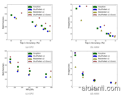 Figure 1: Measurement of accuracy (ImageNet classification on validation set), speed and FLOPs of four network architectures on two hardware platforms with four different level of computation complexities (see text for details). (a, c) GPU results, batchsize=8. (b, d) ARM results, batchsize=1.The best performing algorithm, our proposed ShuffleNet v2, is on the top right region, under all cases.
图1:在具有四个不同计算复杂度的两个硬件平台上,四个网络体系结构的准确性(ImageNet分类在验证集上),速度和FLOP的度量值(有关详细信息,请参见文本)。(a,c)GPU结果,batchsize=8。(b,d)ARM结果,batchsize=1个。在所有情况下,我们建议的ShuffleNet v2是性能最佳的算法。
The discrepancy between the indirect (FLOPs) and direct (speed) metrics can be attributed to two main reasons. First, several important factors that have considerable affection on speed are not taken into account by FLOPs. One such factor is memory access cost (MAC). Such cost constitutes a large portion of runtime in certain operations like group convolution. It could be bottleneck on devices with strong computing power, e.g., GPUs. This cost should not be simply ignored during network architecture design. Another one is degree of parallelism. A model with high degree of parallelism could be much faster than another one with low degree of parallelism, under the same FLOPs.
间接(FLOP)和直接(速度)指标之间的差异可以归因于两个主要原因。首先,FLOP并未考虑对速度有重大影响的几个重要因素。这样的因素之一是内存访问成本(MAC)。在某些操作(例如组卷积)中,此类开销构成了运行时的很大一部分。在具有强大计算能力的设备(例如GPU)上可能会成为瓶颈。在网络体系结构设计期间,不应简单地忽略此成本。另一个是并行度。在相同的FLOP下,具有高并行度的模型可能比具有低并行度的模型快得多。
Second, operations with the same FLOPs could have different running time, depending on the platform. For example, tensor decomposition is widely used in early works [20, 21, 22] to accelerate the matrix multiplication. However, the recent work [19] finds that the decomposition in [22] is even slower on GPU although it reduces FLOPs by 75%. We investigated this issue and found that this is because the latest CUDNN [23] library is specially optimized for 3×3 conv. We cannot certainly think that 3×3 conv is 9 times slower than 1×1 conv.
其次,根据平台的不同,具有相同FLOP的操作可能会具有不同的运行时间。例如,张量分解被广泛应用于早期作品 [ 20,21,22 ],以加速矩阵乘法。然而,最近的工作 [ 19 ]发现[ 22 ]中的分解在GPU上甚至更慢,尽管它可以将FLOP减少75%。我们调查了这个问题,发现这是因为最新的CUDNN [ 23 ]库专门针对3×3转换 我们当然不能认为3×3 转换速度比慢9倍 1×1 转换
With these observations, we propose that two principles should be considered for effective network architecture design. First, the direct metric (e.g., speed) should be used instead of the indirect ones (e.g., FLOPs). Second, such metric should be evaluated on the target platform.
基于这些观察,我们建议为有效的网络体系结构设计应考虑两个原则。首先,应使用直接量度(例如速度)代替间接量度(例如FLOP)。其次,应在目标平台上评估此类指标。
In this work, we follow the two principles and propose a more effective network architecture. In Section 2, we firstly analyze the runtime performance of two representative state-of-the-art networks [15, 14]. Then, we derive four guidelines for efficient network design, which are beyond only considering FLOPs. While these guidelines are platform independent, we perform a series of controlled experiments to validate them on two different platforms (GPU and ARM) with dedicated code optimization, ensuring that our conclusions are state-of-the-art.
在这项工作中,我们遵循这两个原则,并提出了一种更有效的网络体系结构。在第 2,我们首先分析两个有代表性的国家的最先进的网络的运行时性能[ 15,14 ]。然后,我们得出了进行有效网络设计的四项准则,这不仅仅是考虑FLOP。尽管这些准则与平台无关,但我们执行了一系列受控实验,以通过专门的代码优化在两个不同的平台(GPU和ARM)上对它们进行验证,以确保我们的结论是最新的。
In Section 3, according to the guidelines, we design a new network structure. As it is inspired by ShuffleNet [15], it is called ShuffleNet V2. It is demonstrated much faster and more accurate than the previous networks on both platforms, via comprehensive validation experiments in Section 4. Figure 1(a)(b) gives an overview of comparison. For example, given the computation complexity budget of 40M FLOPs, ShuffleNet v2 is 3.5% and 3.7% more accurate than ShuffleNet v1 and MobileNet v2, respectively.
在第3节中 ,根据指南,我们设计了一个新的网络结构。由于它受到ShuffleNet [ 15 ]的启发 ,因此被称为ShuffleNet V2。通过第4节中的全面验证实验,它在两个平台上均比以前的网络更快,更准确地被证明 。图 1(a)(b)给出了比较的概述。例如,给定4000万个FLOP的计算复杂性预算,ShuffleNet v2的准确度分别比ShuffleNet v1和MobileNet v2高3.5%和3.7%。

Figure 2: Run time decomposition on two representative state-of-the-art network architectures, ShuffeNet v1 [15] (1×, g=3) and MobileNet v2 [14] (1×).
图2:两种代表性的最新网络架构*ShufeNet v1 * [ 15 ](1上的运行时分解×, G=3)和*MobileNet v2 * [ 14 ](1×)。
2PRACTICAL GUIDELINES FOR EFFICIENT NETWORK DESIGN 高效网络设计实用指南
Our study is performed on two widely adopted hardwares with industry-level optimization of CNN library. We note that our CNN library is more efficient than most open source libraries. Thus, we ensure that our observations and conclusions are solid and of significance for practice in industry.
我们的研究是在两种广泛采用的硬件上进行的,这些硬件具有CNN库的行业级优化。我们注意到,我们的CNN库比大多数开源库更有效。因此,我们确保我们的观察和结论是可靠的,并且对工业实践具有重要意义。
- GPU. A single NVIDIA GeForce GTX 1080Ti is used. The convolution library is CUDNN 7.0 [23]. We also activate the benchmarking function of CUDNN to select the fastest algorithms for different convolutions respectively.
使用单个NVIDIA GeForce GTX 1080Ti。卷积库为CUDNN 7.0 [ 23 ]。我们还激活CUDNN的基准测试功能,分别为不同的卷积选择最快的算法。
- ARM. A Qualcomm Snapdragon 810. We use a highly-optimized Neon-based implementation. A single thread is used for evaluation.
Qualcomm Snapdragon810。我们使用高度优化的基于Neon的实现。单个线程用于评估。
Other settings include: full optimization options (e.g. tensor fusion, which is used to reduce the overhead of small operations) are switched on. The input image size is 224×224. Each network is randomly initialized and evaluated for 100 times. The average runtime is used.
其他设置包括:启用了完整的优化选项(例如,张量融合,用于减少小操作的开销)。输入图像尺寸为224×224。每个网络都会随机初始化并评估100次。使用平均运行时间。
To initiate our study, we analyze the runtime performance of two state-of-the-art networks, ShuffleNet v1 [15] and MobileNet v2 [14]. They are both highly efficient and accurate on ImageNet classification task. They are both widely used on low end devices such as mobiles. Although we only analyze these two networks, we note that they are representative for the current trend. At their core are group convolution and depth-wise convolution, which are also crucial components for other state-of-the-art networks, such as ResNeXt [7], Xception [12], MobileNet [13], and CondenseNet [16].
为了开始我们的研究,我们分析了两个最新网络ShuffleNet v1 * [ 15 ]和MobileNet v2 * [ 14 ]的运行时性能。它们在ImageNet分类任务上既高效又准确。它们都广泛用于低端设备(例如手机)上。尽管我们仅分析了这两个网络,但我们注意到它们代表了当前的趋势。分组卷积和深度卷积是它们的核心,它们也是其他最新网络的关键组件,例如ResNeXt [ 7 ],Xception [ 12 ],MobileNet [ 13 ]和CondenseNet [ 16 ]。
The overall runtime is decomposed for different operations, as shown in Figure 2. We note that the FLOPs metric only account for the convolution part. Although this part consumes most time, the other operations including data I/O, data shuffle and element-wise operations (AddTensor, ReLU, etc) also occupy considerable amount of time. Therefore, FLOPs is not an accurate enough estimation of actual runtime.
如图2所示,将整个运行时分解为不同的操作 。我们注意到,FLOPs指标仅占卷积部分。尽管这部分消耗大量时间,但其他操作(包括数据I / O,数据混洗和按元素操作(AddTensor,ReLU等))也占用了大量时间。因此,FLOP对实际运行时间的估计不够准确。
Based on this observation, we perform a detailed analysis of runtime (or speed) from several different aspects and derive several practical guidelines for efficient network architecture design.
基于此观察,我们从几个不同方面进行了运行时(或速度)的详细分析,并得出了一些有效的网络体系结构设计的实用指南。
| GPU | (Batches | /sec.) | ARM | (Images | /sec.) | |||
|---|---|---|---|---|---|---|---|---|
| c1:c2 | (c1,c2) for ×1 | ×1 | ×2 | ×4 | (c1,c2) for ×1 | ×1 | ×2 | ×4 |
| 1:1 | (128,128) | 1480 | 723 | 232 | (32,32) | 76.2 | 21.7 | 5.3 |
| 1:2 | (90,180) | 1296 | 586 | 206 | (22,44) | 72.9 | 20.5 | 5.1 |
| 1:6 | (52,312) | 876 | 489 | 189 | (13,78) | 69.1 | 17.9 | 4.6 |
| 1:12 | (36,432) | 748 | 392 | 163 | (9,108) | 57.6 | 15.1 | 4.4 |
Table 1: Validation experiment for Guideline 1. Four different ratios of number of input/output channels (c1 and c2) are tested, while the total FLOPs under the four ratios is fixed by varying the number of channels. Input image size is 56×56.
表1:准则1的验证实验。输入/输出通道数的四种不同比率(C1个 和 C2个)进行测试,而通过改变通道数来固定这四个比率下的总FLOP是固定的。输入图片大小为56×56。
G1) Equal channel width minimizes memory access cost (MAC). The modern networks usually adopt depthwise separable convolutions [12, 13, 15, 14], where the pointwise convolution (i.e., 1×1 convolution) accounts for most of the complexity [15]. We study the kernel shape of the 1×1 convolution. The shape is specified by two parameters: the number of input channels c1 and output channels c2. Let h and w be the spatial size of the feature map, the FLOPs of the 1×1 convolution is B=hwc1c2.
相等的通道宽度可最大程度地减少内存访问成本(MAC)。 现代网络通常采用沿深度可分离卷积 [ 12,13,15,14 ],其中,所述逐点卷积(即,1×1卷积)占了大多数复杂性 [ 15 ]。我们研究了1×1卷积。形状由两个参数指定:输入通道数C1 和输出通道 C2。让H 和 w 是要素图的空间大小,即 1×1 卷积是 B=HwC1C2。
For simplicity, we assume the cache in the computing device is large enough to store the entire feature maps and parameters. Thus, the memory access cost (MAC), or the number of memory access operations, is MAC=hw(c1+c2)+c1c2. Note that the two terms correspond to the memory access for input/output feature maps and kernel weights, respectively.
为简单起见,我们假定计算设备中的缓存足够大,可以存储整个功能图和参数。因此,内存访问成本(MAC)或内存访问操作数为
MAC=hw(c1+c2)+c1c2请注意,这两个术语分别对应于输入/输出特征图和内核权重的内存访问。
From mean value inequality, we have
从均值不平等,我们有
$$MAC =2\sqrt{hwB}+\frac{B}{hw}$$
Therefore, MAC has a lower bound given by FLOPs. It reaches the lower bound when the numbers of input and output channels are equal.
The conclusion is theoretical. In practice, the cache on many devices is not large enough. Also, modern computation libraries usually adopt complex blocking strategies to make full use of the cache mechanism [24]. Therefore, the real MAC may deviate from the theoretical one. To validate the above conclusion, an experiment is performed as follows. A benchmark network is built by stacking 10 building blocks repeatedly. Each block contains two convolution layers. The first contains c1 input channels and c2 output channels, and the second otherwise.
因此,MAC具有FLOP给出的下限。当输入和输出通道数相等时,它达到下限。
结论是理论上的。实际上,许多设备上的缓存不够大。另外,现代计算库通常采用复杂的阻塞策略来充分利用缓存机制[ 24 ]。因此,实际的MAC可能会偏离理论值。为了验证上述结论,进行如下实验。通过重复堆叠10个构建基块来构建基准网络。每个块包含两个卷积层。第一个包含C1个 输入通道和 C2个 输出通道,否则输出第二个通道。
Table 1 reports the running speed by varying the ratio c1:c2 while fixing the total FLOPs. It is clear that when c1:c2 is approaching 1:1, the MAC becomes smaller and the network evaluation speed is faster.
表 1通过改变比率报告了运行速度C1:C2同时固定总FLOP。很明显,当C1:C2 正在接近 1:1,MAC变小,网络评估速度更快。
| GPU | (Batches | /sec.) | ARM | (Images | /sec.) | |||
|---|---|---|---|---|---|---|---|---|
| g | c for ×1 | ×1 | ×2 | ×4 | c for ×1 | ×1 | ×2 | ×4 |
| 1 | 128 | 2451 | 1289 | 437 | 64 | 40.0 | 10.2 | 2.3 |
| 2 | 180 | 1725 | 873 | 341 | 90 | 35.0 | 9.5 | 2.2 |
| 4 | 256 | 1026 | 644 | 338 | 128 | 32.9 | 8.7 | 2.1 |
| 8 | 360 | 634 | 445 | 230 | 180 | 27.8 | 7.5 | 1.8 |
Table 2: Validation experiment for Guideline 2. Four values of group number g are tested, while the total FLOPs under the four values is fixed by varying the total channel number c. Input image size is 56×56.
表2:准则2的验证实验。组号的四个值G 进行测试,同时通过更改总通道数来固定四个值下的总FLOP C。输入图片大小为56×56
G2) Excessive group convolution increases MAC. Group convolution is at the core of modern network architectures [7, 15, 25, 26, 27, 28]. It reduces the computational complexity (FLOPs) by changing the dense convolution between all channels to be sparse (only within groups of channels). On one hand, it allows usage of more channels given a fixed FLOPs and increases the network capacity (thus better accuracy). On the other hand, however, the increased number of channels results in more MAC.
过多的组卷积会增加MAC。 组卷积是现代网络架构的核心 [ 7,15,25,26,27,28 ]。通过更改所有通道之间的稀疏卷积(仅在通道组内),可以降低计算复杂度(FLOP)。一方面,在给定固定FLOP的情况下,它允许使用更多通道,并增加了网络容量(因此具有更高的准确性)。但是,另一方面,增加的通道数将导致更多的MAC。
Formally, following the notations in G1 and Eq. 1, the relation between MAC and FLOPs for 1×1 group convolution is
正式地,遵循G1和Eq中的符号。 1,MAC和FLOP之间的关系1×1分组卷积
$$
MAC =hw(c_{1}+c_{2})+\frac{c_{1}c_{2}}{g}=hwc_{1}+\frac{Bg}{c_{1}}+\frac{B}{hw}
$$
where g is the number of groups and$B=hwc_{1}c_{2}/g$is the FLOPs. It is easy to see that, given the fixed input shape c1×h×w and the computational cost B, MAC increases with the growth of g.
To study the affection in practice, a benchmark network is built by stacking 10 pointwise group convolution layers. Table 2 reports the running speed of using different group numbers while fixing the total FLOPs. It is clear that using a large group number decreases running speed significantly. For example, using 8 groups is more than two times slower than using 1 group (standard dense convolution) on GPU and up to 30% slower on ARM. This is mostly due to increased MAC. We note that our implementation has been specially optimized and is much faster than trivially computing convolutions group by group.
为了在实践中研究这种影响,通过堆叠10个逐点组卷积层来构建基准网络。表 2报告了固定总FLOP时使用不同组号的运行速度。显然,使用较大的组数会显着降低运行速度。例如,在GPU上使用8组的速度比在1组(标准密集卷积)上的速度慢两倍以上,而在ARM上则要慢30%。这主要是由于MAC增加。我们注意到,我们的实现已经过特别优化,并且比逐组轻松地计算卷积要快得多。
Therefore, we suggest that the group number should be carefully chosen based on the target platform and task. It is unwise to use a large group number simply because this may enable using more channels, because the benefit of accuracy increase can easily be outweighed by the rapidly increasing computational cost.
因此,我们建议应根据目标平台和任务谨慎选择组号。使用大的组号是不明智的,因为这可能使使用更多的通道成为可能,因为快速增加的计算成本可以轻易地抵消准确性提高的好处。
| GPU | (Batches | /sec.) | CPU | (Images | /sec.) | |
|---|---|---|---|---|---|---|
| c=128 | c=256 | c=512 | c=64 | c=128 | c=256 | |
| 1-fragment | 2446 | 1274 | 434 | 40.2 | 10.1 | 2.3 |
| 2-fragment-series | 1790 | 909 | 336 | 38.6 | 10.1 | 2.2 |
| 4-fragment-series | 752 | 745 | 349 | 38.4 | 10.1 | 2.3 |
| 2-fragment-parallel | 1537 | 803 | 320 | 33.4 | 9.1 | 2.2 |
| 4-fragment-parallel | 691 | 572 | 292 | 35.0 | 8.4 | 2.1 |
Table 3: Validation experiment for Guideline 3. c denotes the number of channels for 1-fragment. The channel number in other fragmented structures is adjusted so that the FLOPs is the same as 1-fragment. Input image size is 56×56.
表3:准则3的验证实验。C表示1片段的通道数。调整其他分段结构中的通道号,以使FLOP与1-fragment相同。输入图片大小为56×56。
| GPU | (Batches | /sec.) | CPU | (Images | /sec.) | ||
|---|---|---|---|---|---|---|---|
| ReLU | short-cut | c=32 | c=64 | c=128 | c=32 | c=64 | c=128 |
| yes | yes | 2427 | 2066 | 1436 | 56.7 | 16.9 | 5.0 |
| yes | no | 2647 | 2256 | 1735 | 61.9 | 18.8 | 5.2 |
| no | yes | 2672 | 2121 | 1458 | 57.3 | 18.2 | 5.1 |
| no | no | 2842 | 2376 | 1782 | 66.3 | 20.2 | 5.4 |
Table 4: Validation experiment for Guideline 4. The ReLU and shortcut operations are removed from the “bottleneck” unit [4], separately. c is the number of channels in unit. The unit is stacked repeatedly for 10 times to benchmark the speed.
表4:准则4的验证实验。ReLU和快捷方式操作分别从“瓶颈”单元[ 4 ]中删除 。C是单位中的通道数。将该单元重复堆叠10次以测试速度。
G3) Network fragmentation reduces degree of parallelism. In the GoogLeNet series [29, 30, 3, 31] and auto-generated architectures [9, 11, 10]), a “multi-path” structure is widely adopted in each network block. A lot of small operators (called “fragmented operators” here) are used instead of a few large ones. For example, in NASNET-A [9] the number of fragmented operators (i.e. the number of individual convolution or pooling operations in one building block) is 13. In contrast, in regular structures like ResNet [4], this number is 2 or 3.
网络碎片会降低并行度。在GoogLeNet系列 [ 29,30,3,31 ]和自动生成的体系结构 [ 9,11,10 ]),一个“多路径”的结构中的各个网络块被广泛采用。使用了许多小型运算符(在此称为“分段运算符”),而不是一些大型运算符。例如,在*NASNET-A *[ 9 ]中,分段运算符的数量(即,一个构建块中的单个卷积或池化操作的数量)为13。相反,在诸如ResNet [4 ],这个数字是2或3。
Though such fragmented structure has been shown beneficial for accuracy, it could decrease efficiency because it is unfriendly for devices with strong parallel computing powers like GPU. It also introduces extra overheads such as kernel launching and synchronization.
To quantify how network fragmentation affects efficiency, we evaluate a series of network blocks with different degrees of fragmentation. Specifically, each building block consists of from 1 to 4 1×1 convolutions, which are arranged in sequence or in parallel. The block structures are illustrated in appendix. Each block is repeatedly stacked for 10 times. Results in Table 3 show that fragmentation reduces the speed significantly on GPU, e.g. 4-fragment structure is 3× slower than 1-fragment. On ARM, the speed reduction is relatively small.
尽管这种零散的结构已显示出对准确性有利,但由于它对具有强大并行计算能力的设备(如GPU)不友好,因此可能会降低效率。它还引入了额外的开销,例如内核启动和同步。
为了量化网络碎片如何影响效率,我们评估了一系列具有不同碎片度的网络块。具体来说,每个构建块均由1 至 4个 1×1卷积按顺序或并行排列。附录中说明了这些块的结构。每个块重复堆叠10次。表3中的结果 表明,碎片会显着降低GPU的速度,例如4碎片结构为3×比1片段慢。在ARM上,速度降低相对较小。
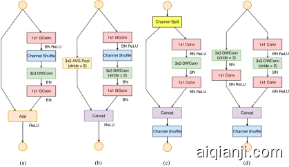
Figure 3: Building blocks of ShuffleNet v1 [15] and this work. (a): the basic ShuffleNet unit; (b) the ShuffleNet unit for spatial down sampling (2×); (c) our basic unit; (d) our unit for spatial down sampling (2×). DWConv: depthwise convolution. GConv: group convolution.
图3:ShuffleNet v1 [ 15 ]的构建块 和这项工作。(a):基本的ShuffleNet单位;(b)用于空间向下采样的ShuffleNet单元(2个×); (c)我们的基本单位;(d)我们用于空间向下采样的单元(2个×)。DWConv:深度卷积。GConv:群卷积。
G4) Element-wise operations are non-negligible. As shown in Figure 2, in light-weight models like [15, 14], element-wise operations occupy considerable amount of time, especially on GPU. Here, the element-wise operators include ReLU, AddTensor, AddBias, etc. They have small FLOPs but relatively heavy MAC. Specially, we also consider depthwise convolution [12, 13, 14, 15] as an element-wise operator as it also has a high MAC/FLOPs ratio.
逐元素运算不可忽略。 如图所示 2,在重量轻的模型,如 [ 15,14 ],逐元素的操作占用相当长的时间,尤其是在GPU。在这里,逐元素运算符包括ReLU,AddTensor,AddBias等。它们的FLOP较小,但MAC相对较重。特别地,我们还考虑深度方向卷积 [ 12,13,14,15 ]作为逐元素操作,因为它也具有较高的MAC / FLOPS比。
For validation, we experimented with the “bottleneck” unit (1×1 conv followed by 3×3 conv followed by 1×1 conv, with ReLU and shortcut connection) in ResNet [4]. The ReLU and shortcut operations are removed, separately. Runtime of different variants is reported in Table 4. We observe around 20% speedup is obtained on both GPU and ARM, after ReLU and shortcut are removed.
为了进行验证,我们尝试了“瓶颈”单元(1×1 转换之后 3×3 转换之后 1×1转换,与ReLU和快捷方式连接)在ResNet [ 4 ]中。ReLU和快捷方式操作将分别删除。表4中报告了不同变体的运行时 。我们观察到,移除ReLU和快捷方式后,GPU和ARM均可实现约20%的加速。
Conclusion and Discussions Based on the above guidelines and empirical studies, we conclude that an efficient network architecture should 1) use ”balanced“ convolutions (equal channel width); 2) be aware of the cost of using group convolution; 3) reduce the degree of fragmentation; and 4) reduce element-wise operations. These desirable properties depend on platform characterics (such as memory manipulation and code optimization) that are beyond theoretical FLOPs. They should be taken into accout for practical network design.
Recent advances in light-weight neural network architectures [15, 13, 14, 9, 11, 10, 12] are mostly based on the metric of FLOPs and do not consider these properties above. For example, ShuffleNet v1 [15] heavily depends group convolutions (against G2) and bottleneck-like building blocks (against G1). MobileNet v2 [14] uses an inverted bottleneck structure that violates G1. It uses depthwise convolutions and ReLUs on “thick” feature maps. This violates G4. The auto-generated structures [9, 11, 10] are highly fragmented and violate G3.
结论与讨论基于上述指导原则和实证研究,我们得出结论,一种有效的网络架构应:1)使用“平衡”卷积(相等的信道宽度);2)注意使用组卷积的代价;3)减少碎片程度;和4)减少按元素操作。这些理想的属性取决于超出平台FLOP的平台特性(例如内存操作和代码优化)。对于实际的网络设计,应该考虑它们。
在重量轻的神经网络结构的最新进展 [ 15,13,14,9,11,10,12 ]大多基于所述度量触发器,并且不考虑上述这些性能。例如,*ShuffleNet v1 * [ 15 ]在很大程度上依赖于组卷积(针对G2)和类似瓶颈的构建块(针对G1)。*MobileNet v2 * [ 14 ]使用了违反G1的倒置瓶颈结构。它在“较厚”特征图上使用深度卷积和ReLU。这违反了G4。自动生成的结构 [ 9,11,10 ]高度分散和违反G3。
Table 5: Overall architecture of ShuffleNet v2, for four different levels of complexities.
表5:ShuffleNet v2的总体体系结构,具有四个不同级别的复杂性。
3SHUFFLENET V2: AN EFFICIENT ARCHITECTURE
Review of ShuffleNet v1 [15]. ShuffleNet is a state-of-the-art network architecture. It is widely adopted in low end devices such as mobiles. It inspires our work. Thus, it is reviewed and analyzed at first.
According to [15], the main challenge for light-weight networks is that only a limited number of feature channels is affordable under a given computation budget (FLOPs). To increase the number of channels without significantly increasing FLOPs, two techniques are adopted in [15]: pointwise group convolutions and bottleneck-like structures. A “channel shuffle” operation is then introduced to enable information communication between different groups of channels and improve accuracy. The building blocks are illustrated in Figure 3(a)(b).
As discussed in Section 2, both pointwise group convolutions and bottleneck structures increase MAC (G1 and G2). This cost is non-negligible, especially for light-weight models. Also, using too many groups violates G3. The element-wise “Add” operation in the shortcut connection is also undesirable (G4). Therefore, in order to achieve high model capacity and efficiency, the key issue is how to maintain a large number and equally wide channels with neither dense convolution nor too many groups.
ShuffleNet v1的评论 [ 15 ]。ShuffleNet是最先进的网络体系结构。它在诸如移动电话之类的低端设备中被广泛采用。它激发了我们的工作。因此,首先要对其进行审查和分析。
根据 [ 15 ],轻量级网络的主要挑战是在给定的计算预算(FLOP)下,仅有限数量的功能通道是可以承受的。为了在不显着增加FLOP的情况下增加通道数量,在[ 15 ]中采用了两种技术 :逐点群卷积和类似瓶颈的结构。然后引入“信道混洗”操作以实现不同组信道之间的信息通信并提高准确性。构造块在图 3(a)(b)中进行了说明。
如第2节所述 ,逐点组卷积和瓶颈结构都增加了MAC(G1和G2)。此费用不可忽略,尤其是对于轻型机型。此外,使用过多的组会违反G3。快捷方式连接中按元素进行“添加”操作也是不希望的(G4)。因此,为了实现较高的模型容量和效率,关键问题是如何保持既不密集卷积又不存在过多组的大量且等宽的信道。
Channel Split and ShuffleNet V2 Towards above purpose, we introduce a simple operator called channel split. It is illustrated in Figure 3(c). At the beginning of each unit, the input of c feature channels are split into two branches with c−c′ and c′ channels, respectively. Following G3, one branch remains as identity. The other branch consists of three convolutions with the same input and output channels to satisfy G1. The two 1×1 convolutions are no longer group-wise, unlike [15]. This is partially to follow G2, and partially because the split operation already produces two groups.
通道拆分和ShuffleNet V2为此,我们引入了一个简单的运算符,称为“通道拆分”。它在图 3(c)中进行了说明。在每个单元的开头,输入C 功能通道分为两个分支 C-C′ 和 C′渠道。在G3之后,保留一个分支作为标识。另一个分支由三个具有相同输入和输出通道的卷积组成,以满足G1。他们俩1个×1个与[ 15 ]不同,卷积不再是按组的 。这部分地遵循G2,部分地因为拆分操作已经产生了两个组。
After convolution, the two branches are concatenated. So, the number of channels keeps the same (G1). The same “channel shuffle” operation as in [15] is then used to enable information communication between the two branches.
After the shuffling, the next unit begins. Note that the “Add” operation in ShuffleNet v1 [15] no longer exists. Element-wise operations like ReLU and depthwise convolutions exist only in one branch. Also, the three successive element-wise operations, “Concat”, “Channel Shuffle” and “Channel Split”, are merged into a single element-wise operation. These changes are beneficial according to G4.
For spatial down sampling, the unit is slightly modified and illustrated in Figure 3(d). The channel split operator is removed. Thus, the number of output channels is doubled.
The proposed building blocks (c)(d), as well as the resulting networks, are called ShuffleNet V2. Based the above analysis, we conclude that this architecture design is highly efficient as it follows all the guidelines.
卷积后,将两个分支连接起来。因此,通道数保持相同(G1)。然后,使用与[ 15 ]中相同的“信道混洗”操作 来启用两个分支之间的信息通信。
改组后,下一个单元开始。请注意,ShuffleNet v1 [ 15 ]中的“添加”操作 不再存在。像ReLU和深度卷积之类的逐元素运算仅存在于一个分支中。同样,三个连续的按元素操作“ Concat”,“ Channel Shuffle”和“ Channel Split”合并为一个按元素操作。根据G4,这些更改是有益的。
对于空间下采样,该单元会稍作修改,如图 3(d)所示。通道拆分运算符已删除。因此,输出通道的数量增加了一倍。
提议的构件(c)(d)以及生成的网络称为ShuffleNet V2。根据以上分析,我们得出结论,此架构设计遵循所有准则,因此非常高效。
The building blocks are repeatedly stacked to construct the whole network. For simplicity, we set c′=c/2. The overall network structure is similar to ShuffleNet v1 [15] and summarized in Table 5. There is only one difference: an additional 1×1 convolution layer is added right before global averaged pooling to mix up features, which is absent in ShuffleNet v1. Similar to [15], the number of channels in each block is scaled to generate networks of different complexities, marked as 0.5×, 1×, etc.
这些构建块被反复堆叠以构建整个网络。为简单起见,我们设置C′=C/2个。总体网络结构类似于ShuffleNet v1 [ 15 ],并在表5中进行了总结 。仅有一个区别:另一个1个×1个卷积层在全局平均池之前添加,以混合功能,而ShuffleNet v1中没有。与[ 15 ]相似,每个块中的通道数按比例缩放以生成不同复杂度的网络,标记为0.5×,1×, 等等。
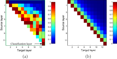
Figure 4: Illustration of the patterns in feature reuse for DenseNet [6] and ShuffleNet V2. (a) (courtesy of [6]) the average absolute filter weight of convolutional layers in a model. The color of pixel (s,l) encodes the average l1-norm of weights connecting layer s to l. (b) The color of pixel (s,l) means the number of channels directly connecting block s to block l in ShuffleNet v2. All pixel values are normalized to [0,1].
图4:DenseNet [ 6 ]和ShuffleNet V2在功能复用中的模式示意图。(a)(由 [ 6 ]提供)模型中卷积层的平均绝对过滤器权重。像素颜色 (s,升) 编码平均值 升1个-权重连接层的范数 s 至 升。(b)像素颜色(s,升)表示直接连接块的通道数s 封锁 升在ShuffleNet v2中。所有像素值均归一化为[0,1个]。
Analysis of Network Accuracy ShuffleNet v2 is not only efficient, but also accurate. There are two main reasons. First, the high efficiency in each building block enables using more feature channels and larger network capacity.
Second, in each block, half of feature channels (when c′=c/2) directly go through the block and join the next block. This can be regarded as a kind of feature reuse, in a similar spirit as in DenseNet [6] and CondenseNet [16].
In DenseNet[6], to analyze the feature reuse pattern, the l1-norm of the weights between layers are plotted, as in Figure 4(a). It is clear that the connections between the adjacent layers are stronger than the others. This implies that the dense connection between all layers could introduce redundancy. The recent CondenseNet [16] also supports the viewpoint.
In ShuffleNet V2, it is easy to prove that the number of “directly-connected” channels between i-th and (i+j)-th building block is rjc, where r=(1−c′)/c. In other words, the amount of feature reuse decays exponentially with the distance between two blocks. Between distant blocks, the feature reuse becomes much weaker. Figure 4(b) plots the similar visualization as in (a), for r=0.5. Note that the pattern in (b) is similar to (a).
Thus, the structure of ShuffleNet V2 realizes this type of feature re-use pattern by design. It shares the similar benefit of feature re-use for high accuracy as in DenseNet [6], but it is much more efficient as analyzed earlier. This is verified in experiments, Table 8.
网络准确性分析ShuffleNet v2不仅效率高,而且准确性高。主要有两个原因。首先,每个构建块中的高效率使得可以使用更多的功能通道和更大的网络容量。
其次,在每个块中,一半的特征通道(当 C′=C/2个)直接穿过该区块并加入下一个区块。与DenseNet [ 6 ]和CondenseNet [ 16 ]相似,这可以看作是一种功能重用。** **
在*DenseNet [ 6 ]中,为了分析特征重用模式,升1个-绘制各层之间的权重范数,如图 4(a)所示。显然,相邻层之间的连接比其他层更牢固。这意味着所有层之间的密集连接可能会引入冗余。最近的CondenseNet * [ 16 ]也支持这种观点。
在ShuffleNet V2中,很容易证明 一世-th和 (一世+Ĵ)第一个构建块是 [RĴC, 在哪里 [R=(1个-C′)/C。换句话说,特征重用量随两个块之间的距离呈指数衰减。在遥远的块之间,功能重用变得很弱。图 4(b)绘制了与(a)中相似的可视化效果,[R=0.5。注意,(b)中的模式类似于(a)。
因此,ShuffleNet V2的结构通过设计实现了这种类型的功能重用模式。与DenseNet * [ 6 ]一样,它也具有重复使用特征以实现高精度的好处*,但是它的效率要高得多。在表8的实验中对此进行了验证。
4EXPERIMENT
Our ablation experiments are performed on ImageNet 2012 classification dataset [32, 33]. Following the common practice [15, 13, 14], all networks in comparison have four levels of computational complexity, i.e. about 40, 140, 300 and 500+ MFLOPs. Such complexity is typical for mobile scenarios. Other hyper-parameters and protocols are exactly the same as ShuffleNet v1 [15].
We compare with following network architectures [12, 14, 6, 15]:
我们的消融实验在ImageNet 2012分类数据集进行 [ 32,33 ]。以下常见的做法 [ 15,13,14 ],在比较所有网络具有四个级别的计算复杂度,即约40,140,300和500 + MFLOPS。这种复杂性对于移动方案而言是典型的。其他超参数和协议与*ShuffleNet v1 *[ 15 ]完全相同。
- ShuffleNet v1 [15]. In [15], a series of group numbers g is compared. It is suggested that the g=3 has better trade-off between accuracy and speed. This also agrees with our observation. In this work we mainly use g=3.
- MobileNet v2 [14]. It is better than MobileNet v1 [13]. For comprehensive comparison, we report accuracy in both original paper [14] and our reimplemention, as some results in [14] are not available.
- Xception [12]. The original Xception model [12] is very large (FLOPs >2G), which is out of our range of comparison. The recent work [34] proposes a modified light weight Xception structure that shows better trade-offs between accuracy and efficiency. So, we compare with this variant.
- DenseNet [6]. The original work [6] only reports results of large models (FLOPs >2G). For direct comparison, we reimplement it following the architecture settings in Table 5, where the building blocks in Stage 2-4 consist of DenseNet blocks. We adjust the number of channels to meet different target complexities.
*ShuffleNet v1 *[ 15 ]。在[ 15 ]中,一系列的组号G比较。建议G=3在精度和速度之间取得更好的权衡。这也与我们的观察一致。在这项工作中,我们主要使用G=3。 - *MobileNet v2 [ 14 ]。它比MobileNet v1 *[ 13 ]更好。为了进行全面比较,我们在原始论文[ 14 ]和重新实现中均报告了准确性 ,因为[ 14 ]中的某些结果 不可用。
- Xception [ 12 ]。原始Xception模型[ 12 ]很大(FLOPs>2G),这超出了我们的比较范围。最近的工作 [ 34 ]提出了一种改进的轻量级Xception结构,该结构在精度和效率之间表现出更好的折衷。因此,我们将其与该变体进行比较。
- DenseNet [ 6 ]。原始工作 [ 6 ]仅报告大型模型(FLOP)的结果>2G)。为了进行直接比较,我们按照表5中的体系结构设置重新实现它,其中阶段2-4中的构建块由DenseNet块组成。我们调整渠道数量以满足不同的目标复杂性。
Table 8 summarizes all the results. We analyze these results from different aspects.
表 8汇总了所有结果。我们从不同方面分析这些结果。
Accuracy vs. FLOPs.
It is clear that the proposed ShuffleNet v2 models outperform all other networks by a large margin22As reported in [14], MobileNet v2 of 500+ MFLOPs has comparable accuracy with the counterpart ShuffleNet v2 (25.3% vs. 25.1% top-1 error); however, our reimplemented version is not as good (26.7% error, see Table 8)., especially under smaller computational budgets. Also, we note that MobileNet v2 performs pooly at 40 MFLOPs level with 224×224 image size. This is probably caused by too few channels. In contrast, our model do not suffer from this drawback as our efficient design allows using more channels. Also, while both of our model and DenseNet [6] reuse features, our model is much more efficient, as discussed in Sec. 3.
Table 8 also compares our model with other state-of-the-art networks including CondenseNet [16], IGCV2 [27], and IGCV3 [28] where appropriate. Our model performs better consistently at various complexity levels.
精度与FLOP的关系。
显然,建议的ShuffleNet v2模型在很大程度上优于所有其他网络22个如[ 14 ]中所述,500多个MFLOP中的MobileNet v2具有与ShuffleNet v2相当的准确性(25.3%对25.1%top-1错误);但是,我们重新实现的版本不是很好(26.7%的错误,请参见表 8)。,尤其是在较小的计算预算下。另外,我们注意到MobileNet v2在40个MFLOP级别上执行池化操作,224×224图片大小。这可能是由于频道太少所致。相比之下,由于我们的高效设计允许使用更多通道,因此我们的模型不会遭受此缺点。而且,虽然我们的模型和DenseNet [ 6 ]都具有重用功能,但是我们的模型效率更高,如Sec中所述。 3。
表 8还将我们的模型与其他最新技术网络进行了比较,包括*CondenseNet * [ 16 ],IGCV2 * [ 27 ]和IGCV3 * [ 28 ]。我们的模型在各种复杂性级别上的性能始终如一。
Inference Speed vs. FLOPs/Accuracy.
For four architectures with good accuracy, ShuffleNet v2, MobileNet v2, ShuffleNet v1 and Xception, we compare their actual speed vs. FLOPs, as shown in Figure 1(c)(d). More results on different resolutions are provided in Appendix Table 1.
ShuffleNet v2 is clearly faster than the other three networks, especially on GPU. For example, at 500MFLOPs ShuffleNet v2 is 58% faster than MobileNet v2, 63% faster than ShuffleNet v1 and 25% faster than Xception. On ARM, the speeds of ShuffleNet v1, Xception and ShuffleNet v2 are comparable; however, MobileNet v2 is much slower, especially on smaller FLOPs. We believe this is because MobileNet v2 has higher MAC (see G1 and G4 in Sec. 2), which is significant on mobile devices.
Compared with MobileNet v1 [13], IGCV2 [27], and IGCV3 [28], we have two observations. First, although the accuracy of MobileNet v1 is not as good, its speed on GPU is faster than all the counterparts, including ShuffleNet v2. We believe this is because its structure satisfies most of proposed guidelines (e.g. for G3, the fragments of MobileNet v1 are even fewer than ShuffleNet v2). Second, IGCV2 and IGCV3 are slow. This is due to usage of too many convolution groups (4 or 8 in [27, 28]). Both observations are consistent with our proposed guidelines.
Recently, automatic model search [9, 10, 11, 35, 36, 37] has become a promising trend for CNN architecture design. The bottom section in Table 8 evaluates some auto-generated models. We find that their speeds are relatively slow. We believe this is mainly due to the usage of too many fragments (see G3). Nevertheless, this research direction is still promising. Better models may be obtained, for example, if model search algorithms are combined with our proposed guidelines, and the direct metric (speed) is evaluated on the target platform.
Finally, Figure 1(a)(b) summarizes the results of accuracy vs. speed, the direct metric. We conclude that ShuffeNet v2 is best on both GPU and ARM.
推理速度与FLOP /精度之间的关系。
对于ShuffleNet v2,MobileNet v2,ShuffleNet v1和Xception等四种精度较高的体系结构,我们将它们的实际速度与FLOP进行比较,如图 1(c)(d)所示。附录表1提供了有关不同分辨率的更多结果。
ShuffleNet v2显然比其他三个网络要快,尤其是在GPU上。例如,在500MFLOP时,ShuffleNet v2比MobileNet v2快58%,比ShuffleNet v1快63%,比Xception快25%。在ARM上,ShuffleNet v1,Xception和ShuffleNet v2的速度是可比的。但是,MobileNet v2的速度要慢得多,尤其是在较小的FLOP上。我们认为这是因为MobileNet v2具有更高的MAC(请参阅第2节中的 G1和G4),这在移动设备上很重要。
与*MobileNet v1 *[ 13 ],*IGCV2 [ 27 ]和IGCV3 *[ 28 ]相比,我们有两个观察结果。首先,尽管MobileNet v1的准确性不高,但它在GPU上的速度要比包括ShuffleNet v2在内的所有同类产品都快。我们认为这是因为其结构可以满足大多数建议的准则(例如,对于G3而言,MobileNet v1的片段比ShuffleNet v2还要少)。其次,IGCV2和IGCV3速度较慢。这是由于4太多卷积组的使用(或8 [ 27,28 ])。两种观察结果均与我们建议的指南一致。
近来,自动模型搜索 [ 9,10,11,35,36,37 ]已成为CNN架构设计一个希望的趋势。表8的底部 评估了一些自动生成的模型。我们发现它们的速度相对较慢。我们认为,这主要是由于使用了太多片段(请参阅G3)。尽管如此,这一研究方向仍然是有前途的。例如,如果将模型搜索算法与我们提出的指南结合起来,并在目标平台上评估直接指标(速度),则可以获得更好的模型。
最后,图 1(a)(b)总结了精度与速度(直接度量)的结果。我们得出的结论是,ShuffeNet v2在GPU和ARM上均是最佳的。
Compatibility with other methods.
ShuffeNet v2 can be combined with other techniques to further advance the performance. When equipped with Squeeze-and-excitation (SE) module [8], the classification accuracy of ShuffleNet v2 is improved by 0.5% at the cost of certain loss in speed. The block structure is illustrated in Appendix Figure 2(b). Results are shown in Table 8 (bottom section).
Generalization to Large Models.
Although our main ablation is performed for light weight scenarios, ShuffleNet v2 can be used for large models (e.g, FLOPs ≥ 2G). Table 6 compares a 50-layer ShuffleNet v2 (details in Appendix) with the counterpart of ShuffleNet v1 [15] and ResNet-50 [4]. ShuffleNet v2 still outperforms ShuffleNet v1 at 2.3GFLOPs and surpasses ResNet-50 with 40% fewer FLOPs.
For very deep ShuffleNet v2 (e.g. over 100 layers), for the training to converge faster, we slightly modify the basic ShuffleNet v2 unit by adding a residual path (details in Appendix). Table 6 presents a ShuffleNet v2 model of 164 layers equipped with SE [8] components (details in Appendix). It obtains superior accuracy over the previous state-of-the-art models [8] with much fewer FLOPs.
与其他方法的兼容性。
ShuffeNet v2可以与其他技术结合使用,以进一步提高性能。当配备挤压和激励(SE)模块 [ 8 ]时,ShuffleNet v2的分类精度提高了0.5%,但代价是速度有所损失。块结构在附录图2(b)中说明。结果示于表 8(底部)。
大型模型的通用化。
尽管我们的主要消融是针对轻型场景进行的,但ShuffleNet v2可以用于大型模型(例如FLOP) ≥2G)。表 6比较了一个50层的ShuffleNet v2(附录中的详细信息)与ShuffleNet v1 [ 15 ]和*ResNet-50 *[ 4 ]的对应关系。ShuffleNet v2在2.3GFLOP的性能上仍胜过ShuffleNet v1,并以40%的FLOP超过了ResNet-50。
对于深度较深的ShuffleNet v2(例如,超过100层),为了加快收敛速度,我们通过添加剩余路径(附录中的详细信息)对基本ShuffleNet v2单元进行了少许修改。表 6列出了配备*SE *[ 8 ]组件的164层ShuffleNet v2模型(详细信息在附录中)。与以前的最新模型[ 8 ]相比,它具有更少的FLOP,从而具有更高的精度。
Object Detection
To evaluate the generalization ability, we also tested COCO object detection [38] task. We use the state-of-the-art light-weight detector – Light-Head RCNN [34] – as our framework and follow the same training and test protocols. Only backbone networks are replaced with ours. Models are pretrained on ImageNet and then finetuned on detection task. For training we use train+val set in COCO except for 5000 images from minival set, and use the minival set to test. The accuracy metric is COCO standard mmAP, i.e. the averaged mAPs at the box IoU thresholds from 0.5 to 0.95.
ShuffleNet v2 is compared with other three light-weight models: Xception [12, 34], ShuffleNet v1 [15] and MobileNet v2 [14] on four levels of complexities. Results in Table 7 show that ShuffleNet v2 performs the best.
Compared the detection result (Table 7) with classification result (Table 8), it is interesting that, on classification the accuracy rank is ShuffleNet v2 ≥ MobileNet v2 > ShuffeNet v1 > Xception, while on detection the rank becomes ShuffleNet v2 > Xception ≥ ShuffleNet v1 ≥ MobileNet v2. This reveals that Xception is good on detection task. This is probably due to the larger receptive field of Xception building blocks than the other counterparts (7 vs. 3). Inspired by this, we also enlarge the receptive field of ShuffleNet v2 by introducing an additional 3×3 depthwise convolution before the first pointwise convolution in each building block. This variant is denoted as ShuffleNet v2*. With only a few additional FLOPs, it further improves accuracy.
We also benchmark the runtime time on GPU. For fair comparison the batch size is set to 4 to ensure full GPU utilization. Due to the overheads of data copying (the resolution is as high as 800×1200) and other detection-specific operations (like PSRoI Pooling [34]), the speed gap between different models is smaller than that of classification. Still, ShuffleNet v2 outperforms others, e.g. around 40% faster than ShuffleNet v1 and 16% faster than MobileNet v2.
Furthermore, the variant ShuffleNet v2* has best accuracy and is still faster than other methods. This motivates a practical question: how to increase the size of receptive field? This is critical for object detection in high-resolution images [39]. We will study the topic in the future.
物体检测
为了评估泛化能力,我们还测试了COCO对象检测[ 38 ]任务。我们使用最先进的轻型检测器– Light-Head RCNN [ 34 ]作为我们的框架,并遵循相同的培训和测试协议。只有骨干网被我们的骨干网取代。在ImageNet上对模型进行预训练,然后根据检测任务对其进行微调。对于训练,我们使用COCO中的train + val设置,除了来自最小设置的5000张图像,然后使用minival进行测试。精度度量标准是COCO标准mmAP,即框IoU阈值处从0.5到0.95的平均mAP。
的ShuffleNet v2是与其他三个轻质机型相比:*Xception *[ 12,34 ],*的ShuffleNet V1 [ 15 ]和MobileNet V2 *[ 14 ]上四个级别的复杂性。表7中的结果 表明ShuffleNet v2表现最佳。
将检测结果(表 7)与分类结果(表 8)进行了比较,有趣的是,分类的准确度等级为ShuffleNet v2≥ MobileNet v2 > ShuffeNet v1 > Xception,在检测到等级后变为ShuffleNet v2 > Xception ≥ ShuffleNet v1 ≥MobileNet v2。这表明Xception在检测任务上很出色。这可能是由于Xception构建块的接受域比其他对应域更大(7 vs. 3)。受此启发,我们还通过引入其他功能扩展了ShuffleNet v2的接受领域3×3在每个构造块中的第一个点状卷积之前进行深度卷积。此变体表示为*ShuffleNet v2 **。仅需几个额外的FLOP,它就可以进一步提高精度。
我们还在GPU上对运行时间进行了基准测试。为了公平比较,批大小设置为4,以确保完全利用GPU。由于数据复制的开销(分辨率高达800×1200)和其他特定于检测的操作(如*PSRoI Pooling *[ 34 ]),不同模型之间的速度差距要小于分类的速度差距。尽管如此,ShuffleNet v2的性能仍优于其他产品,例如,比ShuffleNet v1快40%,比MobileNet v2快16%。
此外,变体ShuffleNet v2 *具有最佳准确性,但仍比其他方法快。这引发了一个实际的问题:如何增加感受野的大小?这对于高分辨率图像中的目标检测至关重要[ 39 ]。将来我们将研究该主题。
| Model | FLOPs | Top-1 err. (%) |
|---|---|---|
| ShuffleNet v2-50 (ours) | 2.3G | 22.8 |
| ShuffleNet v1-50 [15] (our impl.) | 2.3G | 25.2 |
| ResNet-50 [4] | 3.8G | 24.0 |
| SE-ShuffleNet v2-164 (ours, with residual) | 12.7G | 18.56 |
| SENet [8] | 20.7G | 18.68 |
Table 6: Results of large models. See text for details.
表6:大型模型的结果。有关详细信息,请参见文本。
| Model | mmAP | (%) | GPU | Speed | (Images | /sec.) | ||
|---|---|---|---|---|---|---|---|---|
| FLOPs | 40M | 140M | 300M | 500M | 40M | 140M | 300M | 500M |
| Xception | 21.9 | 29.0 | 31.3 | 32.9 | 178 | 131 | 101 | 83 |
| ShuffleNet v1 | 20.9 | 27.0 | 29.9 | 32.9 | 152 | 85 | 76 | 60 |
| MobileNet v2 | 20.7 | 24.4 | 30.0 | 30.6 | 146 | 111 | 94 | 72 |
| ShuffleNet v2 (ours) | 22.5 | 29.0 | 31.8 | 33.3 | 188 | 146 | 109 | 87 |
| ShuffleNet v2* (ours) | 23.7 | 29.6 | 32.2 | 34.2 | 183 | 138 | 105 | 83 |
Table 7: Performance on COCO object detection. The input image size is 800×1200. FLOPs row lists the complexity levels at 224×224 input size. For GPU speed evaluation, the batch size is 4. We do not test ARM because the PSRoI Pooling operation needed in [34] is unavailable on ARM currently.
表7:COCO物体检测的性能。输入图像尺寸为800×1200。FLOPs行列出了以下级别的复杂度224×224输入大小。对于GPU速度评估,批处理大小为4。我们不测试ARM,因为[ 34 ]中所需的PSRoI Pooling操作 当前在ARM上不可用。
5CONCLUSION
| Model | Complexity(MFLOPs) | Top-1err. (%) | GPU Speed (Batches/sec.) | ARM Speed (Images/sec.) |
|---|---|---|---|---|
| ShuffleNet v2 0.5× (ours) | 41 | 39.7 | 417 | 57.0 |
| 0.25 MobileNet v1 [13] | 41 | 49.4 | 502 | 36.4 |
| 0.4 MobileNet v2 [14] (our impl.)* | 43 | 43.4 | 333 | 33.2 |
| 0.15 MobileNet v2 [14] (our impl.) | 39 | 55.1 | 351 | 33.6 |
| ShuffleNet v1 0.5× (g=3) [15] | 38 | 43.2 | 347 | 56.8 |
| DenseNet 0.5× [6] (our impl.) | 42 | 58.6 | 366 | 39.7 |
| Xception 0.5× [12] (our impl.) | 40 | 44.9 | 384 | 52.9 |
| IGCV2-0.25 [27] | 46 | 45.1 | 183 | 31.5 |
| ShuffleNet v2 1× (ours) | 146 | 30.6 | 341 | 24.4 |
| 0.5 MobileNet v1 [13] | 149 | 36.3 | 382 | 16.5 |
| 0.75 MobileNet v2 [14] (our impl.)** | 145 | 32.1 | 235 | 15.9 |
| 0.6 MobileNet v2 [14] (our impl.) | 141 | 33.3 | 249 | 14.9 |
| ShuffleNet v1 1× (g=3) [15] | 140 | 32.6 | 213 | 21.8 |
| DenseNet 1× [6] (our impl.) | 142 | 45.2 | 279 | 15.8 |
| Xception 1× [12] (our impl.) | 145 | 34.1 | 278 | 19.5 |
| IGCV2-0.5 [27] | 156 | 34.5 | 132 | 15.5 |
| IGCV3-D (0.7) [28] | 210 | 31.5 | 143 | 11.7 |
| ShuffleNet v2 1.5× (ours) | 299 | 27.4 | 255 | 11.8 |
| 0.75 MobileNet v1 [13] | 325 | 31.6 | 314 | 10.6 |
| 1.0 MobileNet v2 [14] | 300 | 28.0 | 180 | 8.9 |
| 1.0 MobileNet v2 [14] (our impl.) | 301 | 28.3 | 180 | 8.9 |
| ShuffleNet v1 1.5× (g=3) [15] | 292 | 28.5 | 164 | 10.3 |
| DenseNet 1.5× [6] (our impl.) | 295 | 39.9 | 274 | 9.7 |
| CondenseNet (G=C=8) [16] | 274 | 29.0 | - | - |
| Xception 1.5× [12] (our impl.) | 305 | 29.4 | 219 | 10.5 |
| IGCV3-D [28] | 318 | 27.8 | 102 | 6.3 |
| ShuffleNet v2 2× (ours) | 591 | 25.1 | 217 | 6.7 |
| 1.0 MobileNet v1 [13] | 569 | 29.4 | 247 | 6.5 |
| 1.4 MobileNet v2 [14] | 585 | 25.3 | 137 | 5.4 |
| 1.4 MobileNet v2 [14] (our impl.) | 587 | 26.7 | 137 | 5.4 |
| ShuffleNet v1 2× (g=3) [15] | 524 | 26.3 | 133 | 6.4 |
| DenseNet 2× [6] (our impl.) | 519 | 34.6 | 197 | 6.1 |
| CondenseNet (G=C=4) [16] | 529 | 26.2 | - | - |
| Xception 2× [12] (our impl.) | 525 | 27.6 | 174 | 6.7 |
| IGCV2-1.0 [27] | 564 | 29.3 | 81 | 4.9 |
| IGCV3-D (1.4) [28] | 610 | 25.5 | 82 | 4.5 |
| ShuffleNet v2 2x (ours, with SE [8]) | 597 | 24.6 | 161 | 5.6 |
| NASNet-A [9] ( 4 @ 1056, our impl.) | 564 | 26.0 | 130 | 4.6 |
| PNASNet-5 [10] (our impl.) | 588 | 25.8 | 115 | 4.1 |
Table 8: Comparison of several network architectures over classification error (on validation set, single center crop) and speed, on two platforms and four levels of computation complexity. Results are grouped by complexity levels for better comparison. The batch size is 8 for GPU and 1 for ARM. The image size is 224×224 except: [] 160×160 and [**] 192×192.**表8:在两个平台和四个计算复杂度级别上,几种网络体系结构在分类错误(验证集,单中心作物)和速度方面的比较。将结果按复杂性级别分组,以便更好地进行比较。对于GPU,批处理大小为8;对于ARM,批处理大小为1。图片大小为224×224 除了: [] 160×160 和 [] 192×192。由于目前缺乏有效的实施,我们不提供*CondenseNets [ 16 ]的速度测量。表8:在两个平台和四个计算复杂度级别上,几种网络体系结构在分类错误(验证集,单中心作物)和速度方面的比较。将结果按复杂性级别分组,以便更好地进行比较。对于GPU,批处理大小为8;对于ARM,批处理大小为1。图片大小为224×224 除了: [] 160×160 和 [] 192×192。由于目前缺乏有效的实施,我们不提供*CondenseNets *[ 16 ]的速度测量。
We do not provide speed measurements for CondenseNets [16] due to lack of efficient implementation currently.We propose that network architecture design should consider the direct metric such as speed, instead of the indirect metric like FLOPs. We present practical guidelines and a novel architecture, ShuffleNet v2. Comprehensive experiments verify the effectiveness of our new model. We hope this work could inspire future work of network architecture design that is platform aware and more practical.
我们建议网络体系结构设计应考虑诸如速度之类的直接量度,而不是像FLOPs这样的间接量度。我们提供实用指南和新颖的体系结构ShuffleNet v2。全面的实验证明了我们新模型的有效性。我们希望这项工作能激发人们对平台意识和实用性的网络体系结构设计的未来工作。
Acknowledgements
Thanks Yichen Wei for his help on paper writing. This research is partially supported by National Natural Science Foundation of China (Grant No. 61773229).
感谢魏一尘在论文写作方面的帮助。这项研究得到了中国国家自然科学基金(授权号61773229)的部分支持。
REFERENCES
- [1] Krizhevsky, A., Sutskever, I., Hinton, G.E.: Imagenet classification with deep convolutional neural networks. In: Advances in neural information processing systems. (2012) 1097–1105
- [2] Simonyan, K., Zisserman, A.: Very deep convolutional networks for large-scale image recognition. arXiv preprint arXiv:1409.1556 (2014)
- [3] Szegedy, C., Liu, W., Jia, Y., Sermanet, P., Reed, S., Anguelov, D., Erhan, D., Vanhoucke, V., Rabinovich, A., et al.: Going deeper with convolutions, Cvpr (2015)
- [4] He, K., Zhang, X., Ren, S., Sun, J.: Deep residual learning for image recognition. In: Proceedings of the IEEE conference on computer vision and pattern recognition. (2016) 770–778
- [5] He, K., Zhang, X., Ren, S., Sun, J.: Identity mappings in deep residual networks. In: European Conference on Computer Vision, Springer (2016) 630–645
- [6] Huang, G., Liu, Z., Weinberger, K.Q., van der Maaten, L.: Densely connected convolutional networks. In: Proceedings of the IEEE conference on computer vision and pattern recognition. Volume 1. (2017) 3
- [7] Xie, S., Girshick, R., Dollár, P., Tu, Z., He, K.: Aggregated residual transformations for deep neural networks. In: Computer Vision and Pattern Recognition (CVPR), 2017 IEEE Conference on, IEEE (2017) 5987–5995
- [8] Hu, J., Shen, L., Sun, G.: Squeeze-and-excitation networks. arXiv preprint arXiv:1709.01507 (2017)
- [9] Zoph, B., Vasudevan, V., Shlens, J., Le, Q.V.: Learning transferable architectures for scalable image recognition. arXiv preprint arXiv:1707.07012 (2017)
- [10] Liu, C., Zoph, B., Shlens, J., Hua, W., Li, L.J., Fei-Fei, L., Yuille, A., Huang, J., Murphy, K.: Progressive neural architecture search. arXiv preprint arXiv:1712.00559 (2017)
- [11] Real, E., Aggarwal, A., Huang, Y., Le, Q.V.: Regularized evolution for image classifier architecture search. arXiv preprint arXiv:1802.01548 (2018)
- [12] Chollet, F.: Xception: Deep learning with depthwise separable convolutions. arXiv preprint (2016)
- [13] Howard, A.G., Zhu, M., Chen, B., Kalenichenko, D., Wang, W., Weyand, T., Andreetto, M., Adam, H.: Mobilenets: Efficient convolutional neural networks for mobile vision applications. arXiv preprint arXiv:1704.04861 (2017)
- [14] Sandler, M., Howard, A., Zhu, M., Zhmoginov, A., Chen, L.C.: Inverted residuals and linear bottlenecks: Mobile networks for classification, detection and segmentation. arXiv preprint arXiv:1801.04381 (2018)
- [15] Zhang, X., Zhou, X., Lin, M., Sun, J.: Shufflenet: An extremely efficient convolutional neural network for mobile devices. arXiv preprint arXiv:1707.01083 (2017)
- [16] Huang, G., Liu, S., van der Maaten, L., Weinberger, K.Q.: Condensenet: An efficient densenet using learned group convolutions. arXiv preprint arXiv:1711.09224 (2017)
- [17] Liu, Z., Li, J., Shen, Z., Huang, G., Yan, S., Zhang, C.: Learning efficient convolutional networks through network slimming. In: 2017 IEEE International Conference on Computer Vision (ICCV), IEEE (2017) 2755–2763
- [18] Wen, W., Wu, C., Wang, Y., Chen, Y., Li, H.: Learning structured sparsity in deep neural networks. In: Advances in Neural Information Processing Systems. (2016) 2074–2082
- [19] He, Y., Zhang, X., Sun, J.: Channel pruning for accelerating very deep neural networks. In: International Conference on Computer Vision (ICCV). Volume 2. (2017) 6
- [20] Jaderberg, M., Vedaldi, A., Zisserman, A.: Speeding up convolutional neural networks with low rank expansions. arXiv preprint arXiv:1405.3866 (2014)
- [21] Zhang, X., Zou, J., Ming, X., He, K., Sun, J.: Efficient and accurate approximations of nonlinear convolutional networks. In: Proceedings of the IEEE Conference on Computer Vision and Pattern Recognition. (2015) 1984–1992
- [22] Zhang, X., Zou, J., He, K., Sun, J.: Accelerating very deep convolutional networks for classification and detection. IEEE transactions on pattern analysis and machine intelligence 38(10) (2016) 1943–1955
- [23] Chetlur, S., Woolley, C., Vandermersch, P., Cohen, J., Tran, J., Catanzaro, B., Shelhamer, E.: cudnn: Efficient primitives for deep learning. arXiv preprint arXiv:1410.0759 (2014)
- [24] Das, D., Avancha, S., Mudigere, D., Vaidynathan, K., Sridharan, S., Kalamkar, D., Kaul, B., Dubey, P.: Distributed deep learning using synchronous stochastic gradient descent. arXiv preprint arXiv:1602.06709 (2016)
- [25] Ioannou, Y., Robertson, D., Cipolla, R., Criminisi, A.: Deep roots: Improving cnn efficiency with hierarchical filter groups. arXiv preprint arXiv:1605.06489 (2016)
- [26] Zhang, T., Qi, G.J., Xiao, B., Wang, J.: Interleaved group convolutions for deep neural networks. In: International Conference on Computer Vision. (2017)
- [27] Xie, G., Wang, J., Zhang, T., Lai, J., Hong, R., Qi, G.J.: Igcv 2: Interleaved structured sparse convolutional neural networks. arXiv preprint arXiv:1804.06202 (2018)
- [28] Sun, K., Li, M., Liu, D., Wang, J.: Igcv3: Interleaved low-rank group convolutions for efficient deep neural networks. arXiv preprint arXiv:1806.00178 (2018)
- [29] Szegedy, C., Ioffe, S., Vanhoucke, V., Alemi, A.A.: Inception-v4, inception-resnet and the impact of residual connections on learning. In: AAAI. Volume 4. (2017) 12
- [30] Szegedy, C., Vanhoucke, V., Ioffe, S., Shlens, J., Wojna, Z.: Rethinking the inception architecture for computer vision. In: Proceedings of the IEEE Conference on Computer Vision and Pattern Recognition. (2016) 2818–2826
- [31] Ioffe, S., Szegedy, C.: Batch normalization: Accelerating deep network training by reducing internal covariate shift. In: International conference on machine learning. (2015) 448–456
- [32] Deng, J., Dong, W., Socher, R., Li, L.J., Li, K., Fei-Fei, L.: Imagenet: A large-scale hierarchical image database. In: Computer Vision and Pattern Recognition, 2009. CVPR 2009. IEEE Conference on, IEEE (2009) 248–255
- [33] Russakovsky, O., Deng, J., Su, H., Krause, J., Satheesh, S., Ma, S., Huang, Z., Karpathy, A., Khosla, A., Bernstein, M., et al.: Imagenet large scale visual recognition challenge. International Journal of Computer Vision 115(3) (2015) 211–252
- [34] Li, Z., Peng, C., Yu, G., Zhang, X., Deng, Y., Sun, J.: Light-head r-cnn: In defense of two-stage object detector. arXiv preprint arXiv:1711.07264 (2017)
- [35] Xie, L., Yuille, A.: Genetic cnn. arXiv preprint arXiv:1703.01513 (2017)
- [36] Real, E., Moore, S., Selle, A., Saxena, S., Suematsu, Y.L., Le, Q., Kurakin, A.: Large-scale evolution of image classifiers. arXiv preprint arXiv:1703.01041 (2017)
- [37] Zoph, B., Le, Q.V.: Neural architecture search with reinforcement learning. arXiv preprint arXiv:1611.01578 (2016)
- [38] Lin, T.Y., Maire, M., Belongie, S., Hays, J., Perona, P., Ramanan, D., Dollár, P., Zitnick, C.L.: Microsoft coco: Common objects in context. In: European conference on computer vision, Springer (2014) 740–755
- [39] Peng, C., Zhang, X., Yu, G., Luo, G., Sun, J.: Large kernel matters–improve semantic segmentation by global convolutional network. arXiv preprint arXiv:1703.02719 (2017)
APPENDIX
 Figure 1: Building blocks used in experiments for guideline 3. (a) 1-fragment. (b) 2-fragment-series. (c) 4-fragment-series. (d) 2-fragment-parallel. (e) 4-fragment-parallel.| | | | GPU (Batches/sec.) | CPU (Images/sec.) |
| - | - | - | - |
| Input size | FLOPs | 40M | 140M | 300M | 500M | 40M | 140M | 300M | 500M |
| 320x320 | ShuffleNet v2 | 315∗ | 525 | 474 | 422 | 28.1 | 12.5 | 6.1 | 3.4 |
| ShuffleNet v1 | 236∗ | 414 | 344 | 275 | 27.2 | 11.4 | 5.1 | 3.1 |
| MobileNet v2 | 187∗ | 460 | 389 | 335 | 11.4 | 6.4 | 4.6 | 2.7 |
| Xception | 279∗ | 463 | 408 | 350 | 31.1 | 10.1 | 5.6 | 3.5 |
| 640x480 | ShuffleNet v2 | 424 | 394 | 297 | 250 | 9.3 | 4.0 | 1.9 | 1.1 |
| ShuffleNet v1 | 396 | 269 | 198 | 156 | 8.0 | 3.7 | 1.6 | 1.0 |
| MobileNet v2 | 338 | 248 | 208 | 165 | 3.8 | 2.0 | 1.4 | 0.8 |
| Xception | 399 | 326 | 244 | 209 | 9.6 | 3.2 | 1.7 | 1.1 |
| 1080x720 | ShuffleNet v2 | 248 | 197 | 141 | 115 | 3.5 | 1.5 | 0.7 | 0.4 |
| ShuffleNet v1 | 203 | 131 | 96 | 77 | 2.9 | 1.4 | 0.4 | 0.3 |
| MobileNet v2 | 159 | 117 | 99 | 78 | 1.4 | 0.7 | 0.3 | 0.3 |
| Xception | 232 | 160 | 124 | 106 | 3.6 | 1.2 | 0.5 | 0.4 |
(a) Comparison of actual speeds (whole architecture). | | | | GPU (Batches/sec.) | CPU (Images/sec.) |
| - | - | - | - |
| Input size | Channel (c) for ShuffleNet v2 | c=64 | c=128 | c=256 | c=64 | c=128 | c=256 |
| 56x56 | ShuffleNet v2 | 216 | 142 | 81 | 34.8 | 12.3 | 3.9 |
| ShuffleNet v1 | 127 | 73 | 45 | 24.3 | 9.4 | 3.0 |
| MobileNet v2 | 89 | 125 | 69 | 25.8 | 10.0 | 3.0 |
| Xception | 185 | 52 | 68 | 27.0 | 9.7 | 3.1 |
| 28x28 | ShuffleNet v2 | 407 | 313 | 237 | 174.5 | 53.4 | 16.6 |
| ShuffleNet v1 | 298 | 222 | 60 | 139.7 | 43.9 | 13.2 |
| MobileNet v2 | 381 | 286 | 189 | 118.3 | 46.2 | 13.3 |
| Xception | 254 | 238 | 169 | 117.0 | 45.8 | 14.0 |
| (b) Comparison of actual speeds (units). |
|---|
Table 1: Table (a) compares the speed of each network (whole architecture). Table (b) compares the speed of each network’s unit, we stack 10 network units of each network; the value of c means the number of channels for ShuffleNet v2, we adjust the number of channels to keep the FLOPs unchanged for other network units. Please refer to Section 4 for details. [∗] For the models of 40M FLOPs with input size of 320×320, the batchsize is set to 8 to ensure the GPU utilization rate, and we set batchsize=1 otherwise.| layer | | output |
| - |
| size |
| | ShuffleNet v1-50 |
| - |
| (group=3) |
| ShuffleNet v2-50 | Resnet-50 | | SE-ShuffleNet |
| - |
| v2-164 |
| conv1_x | 112×112 | 3×3, 64, stride 2 | 3×3, 64, stride 2 | 7×7, 64, stride 2 | |
| - | |||||
| 3×3, 64 | |||||
| 3×3, 128 |
|
| conv2_x | 56×56 | 3×3 max pool, stride 2 |
| ×3 | ×3 | ×3 | ×10 |
| conv3_x | 28×28 | ×4 | ×4 | ×4 | ×10 |
| conv4_x | 14×14 | ×6 | ×6 | ×6 | ×23 |
| conv5_x | 7×7 | ×3 | ×3 | ×3 | ×10 |
| conv6 | 7×7 | - | 1×1, 2048 | - | 1×1, 2048 |
| | 1×1 | average pool, 1000-d fc, softmax |
| FLOPs | 2.3G | 2.3G | 3.8G | 12.7G |
Table 2: Architectures for large models. Building blocks are shown in brackets, with the convolution kernel shapes and the numbers of blocks stacked. Downsampling is performed by conv3_1,conv4_1, and conv5_1 with a stride of 2. For ShuffleNet v1-50 and ResNet-50, the bottleneck ratio is set to 1:4. For SE-ShuffleNet v2-164, we add the SE modules right before the residual add-ReLUs (details in Appendix Figure 2); we set the neural numbers in SE modules to the 1/2 of the channel numbers in the corresponding building blocks. See Section 4 for details. Figure 2: Building blocks of ShuffleNet v2 with SE/residual. (a) ShuffleNet v2 with residual. (b) ShuffleNet v2 with SE. (c) ShuffleNet v2 with SE and residual.