Diffusion Models without Classifier-free Guidance
无需无分类器指导的扩散模型
Zhicong Tang 1 Jianmin Bao? Dong Chen? Baining Guo2
Zhicong Tang 1 Jianmin Bao? Dong Chen? Baining Guo2
Abstract
摘要
This paper presents Model-guidance (MG), a novel objective for training diffusion model that addresses and removes of the commonly used Classifier-free guidance (CFG). Our innovative approach transcends the standard modeling of solely data distribution to incorporating the posterior probability of conditions. The proposed technique originates from the idea of CFG and is easy yet effective, making it a plug-and-play module for existing models. Our method significantly accelerates the training process, doubles the inference speed, and achieve exceptional quality that parallel and even surpass concurrent diffusion models with CFG. Extensive experiments demonstrate the effectiveness, efficiency, s cal ability on different models and datasets.Finally, we establish state-of-theart performance on ImageNet 256 benchmarks with an FID of 1.34.Our code is available at qithub.com/tzco/Diffusion-wo-CFG.
本文提出了模型引导 (Model-guidance, MG),这是一种用于训练扩散模型的新目标,旨在解决并替代常用的无分类器引导 (Classifier-free guidance, CFG)。我们的创新方法超越了仅对数据分布进行标准建模的方式,转而结合了条件的后验概率。该技术源自 CFG 的思想,简单而有效,使其成为现有模型的即插即用模块。我们的方法显著加速了训练过程,将推理速度提高了一倍,并实现了与甚至超越使用 CFG 的并行扩散模型的卓越质量。大量实验证明了该方法在不同模型和数据集上的有效性、效率和可扩展性。最终,我们在 ImageNet 256 基准测试中建立了最先进的性能,FID 达到 1.34。我们的代码可在 qithub.com/tzco/Diffusion-wo-CFG 获取。

Figure 1: We propose Model-guidance (MG), removing Classifier-free guidance (CFG) for diffusion models and achieving state-of-the-art on ImageNet with FID of 1.34. (a) Instead of running models twice during inference (green and red), MG directly learns the final distribution (blue). (b) MG requires only one line of code modification while providing excellent improvements. (c) Comparing to concurrent methods, MG yields lowest FID even without CFG.
图 1: 我们提出了模型指导 (Model-guidance, MG),去除了扩散模型中的无分类器指导 (Classifier-free guidance, CFG),并在 ImageNet 上实现了 FID 为 1.34 的最先进性能。(a) 与在推理过程中运行模型两次 (绿色和红色) 不同,MG 直接学习最终分布 (蓝色)。(b) MG 只需修改一行代码即可提供显著的改进。(c) 与并行方法相比,即使没有 CFG,MG 也能产生最低的 FID。
1. Introduction
1. 引言
Diffusion models (Sohl-Dickstein et al., 2015; Song & Ermon, 2019; Ho et al., 2020; Song et al., 2021a;b) have become the cornerstone of many successful generative models, e.g. image generation (Dhariwal & Nichol, 2021; Nichol et al., 2022; Rombach et al., 2022; Podell et al., 2024; Chen et al., 2024) and video generation (Ho et al., 2022; Blattmann et al., 2023; Gupta et al., 2025; Polyak et al., 2024; Wang et al., 2024) tasks. However, diffusion models also struggle to generate “low temperature” samples (Ho & Salimans, 2021; Karras et al., 2024) due to the nature of training objectives, and techniques such as Classifier guidance (Dhariwal & Nichol, 2021) and Classifier-free guidance (CFG) (Ho & Salimans, 2021) are proposed to improve performances.
扩散模型 (Sohl-Dickstein et al., 2015; Song & Ermon, 2019; Ho et al., 2020; Song et al., 2021a;b) 已成为许多成功的生成模型的基石,例如图像生成 (Dhariwal & Nichol, 2021; Nichol et al., 2022; Rombach et al., 2022; Podell et al., 2024; Chen et al., 2024) 和视频生成 (Ho et al., 2022; Blattmann et al., 2023; Gupta et al., 2025; Polyak et al., 2024; Wang et al., 2024) 任务。然而,由于训练目标的性质,扩散模型也难以生成“低温”样本 (Ho & Salimans, 2021; Karras et al., 2024),因此提出了分类器引导 (Dhariwal & Nichol, 2021) 和无分类器引导 (CFG) (Ho & Salimans, 2021) 等技术来提高性能。
Despite its advantage and ubiquity, CFG has several drawbacks (Karras et al., 2024) and poses challenges to effective implementations (Ky nk a an niemi et al., 2024) of diffusion models. One critical limitation is the simultaneous training of unconditional model apart from the main diffusion model. The unconditional model is typically implemented by randomly dropping the condition of training pairs and replacing with an manually defined empty label. The introduction of additional tasks may reduce network capabilities and lead to skewed sampling distributions (Karras et al., 2024; Ky nk a an niemi et al., 2024). Furthermore, CFG requires two forward passes per denoising step during inference, one for the conditioned and another for the un conditioned model, thereby significantly escalating the computational costs.
尽管 CFG 具有优势和普遍性,但它也存在一些缺点 (Karras et al., 2024) ,并对扩散模型的有效实现提出了挑战 (Ky nk a an niemi et al., 2024) 。一个关键局限性是除了主扩散模型外,还需要同时训练无条件模型。无条件模型通常通过随机丢弃训练对的条件并替换为手动定义的空标签来实现。引入额外任务可能会降低网络能力,并导致采样分布偏差 (Karras et al., 2024; Ky nk a an niemi et al., 2024) 。此外,CFG 在推理过程中每个去噪步骤需要两次前向传递,一次用于条件模型,另一次用于无条件模型,从而显著增加了计算成本。
In this work, we propose Model-guidance (MG), an innovative method for diffusion models to effectively circumvent CFG and boost performances, thereby eliminating the limitations above. We propose a novel objective that transcends from simply modeling the data distribution to incorporating the posterior probability of conditions. Specifically, we leverage the model itself as an implicit classifier and directly learn the score of calibrated distribution during training.
在本工作中,我们提出了模型引导 (Model-guidance, MG),这是一种创新的扩散模型方法,能够有效规避 CFG 并提升性能,从而消除上述限制。我们提出了一种新的目标,它超越了简单的数据分布建模,转而结合条件后验概率。具体而言,我们利用模型本身作为隐式分类器,并在训练过程中直接学习校准分布的得分。
As depicted in Figure 1, our proposed method confers multiple substantial breakthroughs. First, it significantly refines generation quality and accelerates training processes, with experiments showcasing $\mathrm{a}\geq,6.5\times$ convergence speedup than vanilla diffusion models with excellent quality. Second, the inference speed is doubled with our method, as each denoising step needs only one network forward in contrast to two in CFG. Besides, it is easy to implement and requires only one line of code modification, making it a plug-and-play module of existing diffusion models with instant improvements. Finally, it is an end-to-end method that excels traditional two-stage distillation-based approaches and even outperforms CFG in generation performances.
如图 1 所示,我们提出的方法带来了多项重大突破。首先,它显著提高了生成质量并加速了训练过程,实验表明其收敛速度比普通扩散模型快 $\mathrm{a}\geq,6.5\times$,且质量优异。其次,使用我们的方法推理速度翻倍,因为每个去噪步骤只需要一次网络前向传播,而 CFG 需要两次。此外,它易于实现,只需修改一行代码,使其成为现有扩散模型的即插即用模块,能够立即带来改进。最后,它是一种端到端的方法,优于传统的基于两阶段蒸馏的方法,甚至在生成性能上超越了 CFG。
We conduct comprehensive experiments on the prevalent Imagenet (Deng et al., 2009; Russ a kov sky et al., 2015) benchmarks with $256!\times!256$ and $512!\times!512$ resolution and compare with a wide variates of concurrent models to attest the effec ti ve ness of our proposed method. The evaluation results demonstrate that our method not only parallels and even outperforms other approaches with CFG, but also scales to different models and datasets, making it a promising enhancement for diffusion models. In conclusion, we make the following contribution in this work:
我们在流行的 Imagenet (Deng et al., 2009; Russakovsky et al., 2015) 基准上进行了全面的实验,分辨率为 $256!\times!256$ 和 $512!\times!512$,并与多种同期模型进行了比较,以证明我们提出方法的有效性。评估结果表明,我们的方法不仅与 CFG 的其他方法相当甚至超越,还能扩展到不同的模型和数据集,使其成为扩散模型的有力增强。总之,我们在这项工作中做出了以下贡献:
· We proposed a novel and effective method, Modelguidance (MG), for training diffusion models. · MG removes CFG for diffusion models and greatly accelerates both training and inference process. · Extensive experiments with SOTA results on ImageNet demonstrate the usefulness and advantages of MG.
· 我们提出了一种新颖且有效的方法,Modelguidance (MG),用于训练扩散模型。
· MG 移除了扩散模型中的 CFG,并大幅加速了训练和推理过程。
· 在 ImageNet 上进行的广泛实验及 SOTA 结果证明了 MG 的有效性和优势。
2. Background
2. 背景
2.1. Diffusion and Flow Models
2.1. 扩散和流模型
Diffusion models (Sohl-Dickstein et al., 2015; Song & Ermon, 2019; Ho et al., 2020; Song et al., 2021a;b) are a class of generative models that utilize forward and reverse stochastic processes to model complex data distributions.
扩散模型 (Sohl-Dickstein et al., 2015; Song & Ermon, 2019; Ho et al., 2020; Song et al., 2021a;b) 是一类生成式模型,利用正向和反向随机过程来建模复杂的数据分布。
The forward process adds noise and transforms data samples into Gaussian distributions as
前向过程通过添加噪声将数据样本转换为高斯分布

where $x_{t}$ represents the noised data at timestep $t$ and $\bar{\alpha}{t}=$ $\textstyle\prod{s=1}^{t}\alpha_{s}$ is the noise schedule.
其中 $x_{t}$ 表示时间步 $t$ 的加噪数据,$\bar{\alpha}{t}=$ $\textstyle\prod{s=1}^{t}\alpha_{s}$ 表示噪声调度。
Conversely, the reverse process learns to denoise and finally recover the original data distribution, which aims to reconstruct score (Sohl-Dickstein et al., 2015; Song et al., 2021b) from the noisy samples $x_{t}$ by learning
相反,反向过程通过学习从噪声样本 $x_{t}$ 中重建得分 (Sohl-Dickstein et al., 2015; Song et al., 2021b),从而去噪并最终恢复原始数据分布。

where $\mu_{\theta}$ and $\Sigma_{\theta}$ are mean and variance and commonly predicted by neural networks.
其中 $\mu_{\theta}$ 和 $\Sigma_{\theta}$ 是均值和方差,通常由神经网络预测。
In common implementations, the training of diffusion mod.
在常见实现中,扩散模型的训练。
els leverages a re-parameterized objective that directly pre- dicts the noise at each step (Ho et al., 2020)
els 利用了一种重新参数化的目标,直接预测每一步的噪声 (Ho et al., 2020)

where $x_{t}$ is derived from the forward process in Equation (1) with $x_{0}$ and $\epsilon$ drawn from dataset and Gaussian noises.
其中 $x_{t}$ 是由公式 (1) 中的前向过程推导得出,$x_{0}$ 和 $\epsilon$ 分别从数据集和高斯噪声中抽取。
Conditional diffusion models allow users to generate samples aligned with specified demands and precisely control the contents of samples. In this case, the generation process is manipulated with give conditions $c$ , such as class labels or text prompts, where network functions are $\epsilon_{\theta}(x_{t},t,c)$
条件扩散模型允许用户生成符合指定需求的样本,并精确控制样本内容。在这种情况下,生成过程通过给定的条件 $c$ 进行操控,例如类别标签或文本提示,其中网络函数为 $\epsilon_{\theta}(x_{t},t,c)$。
Flow Models (Lipman et al., 2023; Liu et al., 2023; Albergo et al., 2023; Tong et al., 2024) are another emerging type of generative models similar to diffusion models. Flow models utilize the concept of Ordinary Differential Equations (ODEs) to bridge the source and target distribution and learn the directions from noise pointing to ground-truth data.
流模型 (Lipman et al., 2023; Liu et al., 2023; Albergo et al., 2023; Tong et al., 2024) 是另一种新兴的生成模型,类似于扩散模型。流模型利用常微分方程 (ODEs) 的概念来连接源分布和目标分布,并学习从噪声指向真实数据的方向。
The forward process of fow models is defined as an Optimal Transport (OT) interpol ant (McCann, 1997)
前向过程由最优传输 (Optimal Transport, OT) 插值 (McCann, 1997) 定义

and the loss function takes the form (Lipman et al., 2023)
损失函数的形式为 (Lipman et al., 2023)

where the ground-truth conditional flow is given by
其中真实条件流由

2.2. Classifier-Free Guidance
2.2. 无分类器引导
Classifier-free guidance (CFG) (Ho & Salimans, 2021) is a widely adopted technique in conditional diffusion models to enhance generation performance and alignment to conditions. It provides an explicit control of the focus on conditioning variables and avoids to sample within the "low temperature” regions with low quality.
无分类器引导 (Classifier-free guidance, CFG) (Ho & Salimans, 2021) 是一种在条件扩散模型中广泛采用的技术,用于增强生成性能和对条件的对齐。它提供了对条件变量焦点的显式控制,并避免了在低质量的“低温”区域进行采样。
The key design of CFG is to combine the posterior probability and utilize Bayes’ rule during inference time. To facilitate this, it is required to train both conditional and unconditional diffusion models. In particular, CFG trains the models to predict
CFG 的关键设计是在推理时结合后验概率并利用贝叶斯规则。为了实现这一点,需要同时训练条件扩散模型和无条件扩散模型。具体而言,CFG 训练模型以进行预测
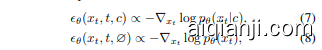
where is an additional empty class introduced in common practices. During training, the model switches between the two modes with a ratio $\lambda$
其中 $\lambda$ 是在常见实践中引入的额外空类。在训练期间,模型以 $\lambda$ 的比例在两种模式之间切换。
For inference, the model combines the conditional and unconditional scores and guides the denoising process as
在推理过程中,模型结合条件和非条件分数,并指导去噪过程
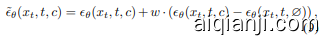

where $w$ is the guidance scale that controls the focus on conditional scores and the trade-off between generation performance and sampling diversity. CFG has become an widely adopted protocol in most of diffusion models for tasks, such as image generation and video generation.
其中,$w$ 是控制条件分数关注度以及生成性能与采样多样性之间权衡的指导尺度。CFG 已成为大多数扩散模型在图像生成和视频生成等任务中广泛采用的协议。
2.3. Distillation-based Methods
2.3. 基于蒸馏的方法
Besides acceleration (Song et al., 2023), researchers (Sauer et al., 2024) also adopt distillation on diffusion models with CFG to improve sampling quality. Rectified Flow (Liu et al., 2023) disentangles generation trajectories and streamline learning difficulty by alternatively using offline model to provide training pairs for online models. Distillation is also used to learn a smaller one-step model to match the generation performance of larger multi-step models (Meng et al., 2023). Pioneering diffusion models (Black-Forest-Labs, 2024; Stability-AI, 2024) are released with a distillate d version, where CFG scale is viewed as an additional embedding to provide accurate control. However, these approaches involve two-stage learning and require extra computation and storage for offline teacher models.
除了加速 (Song et al., 2023) 之外,研究人员 (Sauer et al., 2024) 还在带有 CFG 的扩散模型上采用蒸馏技术以提高采样质量。Rectified Flow (Liu et al., 2023) 通过交替使用离线模型为在线模型提供训练对,解耦生成轨迹并简化学习难度。蒸馏也被用于学习更小的一步模型,以匹配更大规模多步模型的生成性能 (Meng et al., 2023)。开创性的扩散模型 (Black-Forest-Labs, 2024; Stability-AI, 2024) 发布了蒸馏版本,其中 CFG 尺度被视为额外的嵌入,以提供精确控制。然而,这些方法涉及两阶段学习,并且需要为离线教师模型提供额外的计算和存储。
3. Method
3. 方法
3.1. Rethinking Classifier-free guidance
3.1. 重新思考无分类器引导
Due to the complex nature of visual datasets, diffusion mod- els often struggle whether to recover real image distribution or engage in the alignment to conditions. Classifier-free guidance (CFG) is then proposed and has become an indispensable ingredient of modern diffusion models (Nichol & Dhariwal, 2021; Karras et al., 2022; Saharia et al.,2022;
由于视觉数据集的复杂性,扩散模型(Diffusion Models)往往难以在恢复真实图像分布和满足条件对齐之间做出选择。因此,无分类器引导(Classifier-Free Guidance, CFG)被提出,并已成为现代扩散模型中不可或缺的组成部分(Nichol & Dhariwal, 2021; Karras et al., 2022; Saharia et al., 2022)。
Figure 2: We use a grid 2D distribution with two classes, marked with orange and gray regions, as example and train diffusion models on it. We plot the generated samples, trajectories, and probability density function (PDF) of conditional, unconditional, CFG-guided model, and our approach. (a) The first row indicates that although CFG improves quality by eliminating outliers, the samples concentrate in the center of data distributions, resulting the loss of diversity. In contrast, our method yields less outliers than the conditional model and a better coverage of data than CFG. (b) In the second row, the trajectories of CFG show sharp turns at the beginning, e.g. samples inside the red box, while our method directly drives the samples to the closet data distributions. (c) The PDF plots of the last row also suggest that our method predicts more symmetric contours than CFG, balancing both quality and diversity.
图 2: 我们使用一个带有两个类别的网格 2D 分布(用橙色和灰色区域标记)作为示例,并在其上训练扩散模型。我们绘制了生成样本、轨迹以及条件模型、无条件模型、CFG 引导模型和我们方法的概率密度函数 (PDF)。(a) 第一行表明,尽管 CFG 通过消除异常值提高了质量,但样本集中在数据分布的中心,导致多样性的丧失。相比之下,我们的方法产生的异常值比条件模型更少,并且比 CFG 更好地覆盖了数据。(b) 在第二行中,CFG 的轨迹在开始时显示出急剧的转弯(例如红色框内的样本),而我们的方法直接将样本驱动到最近的数据分布。(c) 最后一行的 PDF 图也表明,我们的方法比 CFG 预测出更对称的轮廓,平衡了质量和多样性。
Hoogeboom et al., 2023). It drives the sample towards the regions with higher likelihood of conditions with Equation (9), where the images are more canonical and better modeled by networks (Karras et al., 2024).
Hoogeboom 等人, 2023)。它通过公式 (9) 将样本驱动到条件可能性更高的区域,这些区域的图像更规范且更容易被网络建模 (Karras 等人, 2024)。
However, CFG has with several disadvantages (Karras et al., 2024; Ky nk a an niemi et al., 2024), such as the multitask learning of both conditional and unconditional generation, and the doubled number of function evaluations (NFEs) during inference. Moreover, the tempting property that solving the denoising process according to Equation (9) eventually recovers data distribution does not hold, as the joint distribution does not represent a valid heat diffusion of the ground-truth (Zheng & Lan, 2024). This results in exaggerated truncation and mode dropping similar to (Karras et al., 2018; Brock et al., 2019; Sauer et al., 2022), since the samples are blindly pushed towards the regions with higher posterior probability. The generation trajectories are distorted in Section 1, the images are often over-saturated in color, and the content of samples is overly simplified.
然而,CFG 存在一些缺点 (Karras et al., 2024; Ky nk a an niemi et al., 2024),例如同时进行条件生成和无条件生成的多任务学习,以及在推理过程中函数评估次数 (NFEs) 翻倍。此外,根据公式 (9) 解决去噪过程最终恢复数据分布的诱人特性并不成立,因为联合分布并不代表真实数据的热扩散 (Zheng & Lan, 2024)。这导致了类似于 (Karras et al., 2018; Brock et al., 2019; Sauer et al., 2022) 的过度截断和模式丢失,因为样本被盲目推向具有更高后验概率的区域。在第 1 节中,生成轨迹被扭曲,图像颜色往往过饱和,样本内容过于简化。
CFG originates from the classifier-guidance (Dhariwal & Nichol, 2021) that incorporates an auxiliary classifier model $p_{\theta}\big(c|x_{t}\big)$ to modify the sampling distribution as
CFG 源自分类器引导 (classifier-guidance) (Dhariwal & Nichol, 2021),它通过引入辅助分类器模型 $p_{\theta}\big(c|x_{t}\big)$ 来调整采样分布为

and estimates the posterior probability term with Bayes’ rule
并使用贝叶斯规则估计后验概率项

where $p_{\theta}(\boldsymbol{x}{t}|\boldsymbol{c})$ and $p{\theta}{\left(x_{t}\right)}$ are conditional and unconditional distributions, respectively.
其中 $p_{\theta}(\boldsymbol{x}{t}|\boldsymbol{c})$ 和 $p{\theta}{\left(x_{t}\right)}$ 分别表示条件分布和无条件分布。
The unconditional model is usually implemented by randomly replacing labels by an empty class with a ratio $\lambda$ During inference, each sample is typically forwarded twice, one with and one without conditions. The finding naturally leads us to the question: can we fuse the auxiliary classifier into diffusion models in a more effcient and elegant way?
无条件模型通常通过以一定比例 $\lambda$ 随机将标签替换为空类来实现。在推理过程中,每个样本通常会被前向传播两次,一次带条件,一次不带条件。这一发现自然引出了一个问题:我们能否以更高效和优雅的方式将辅助分类器融入到扩散模型中?

Figure 3: I lust ration of our method. (a) The green and red arrow point towards the centroids of data distributions, as the training pairs $(x_{0},\epsilon)$ are randomly sampled. (b) While CFG provides accurate directions by subtracting the two vectors, our method directly learns the blue arrow, $\nabla\log\tilde{p}{\theta}(x{t}|c)$
图 3: 我们的方法示意图。(a) 绿色和红色箭头指向数据分布的质心,训练对 $(x_{0},\epsilon)$ 是随机采样的。(b) 虽然 CFG 通过减去两个向量提供准确的方向,但我们的方法直接学习蓝色箭头 $\nabla\log\tilde{p}{\theta}(x{t}|c)$
3.2. Model-guidance Loss
3.2. 模型引导损失
Conditional diffusion models optimize the conditional probability $p_{\theta}(\boldsymbol{x}{t}|\boldsymbol{c})$ by Equation (3), where $x{t}$ is the noisy data and $c$ is the condition, e.g. , labels and prompts. However, the models tend to ignore the condition in common practices and CFG (Ho et al., 2020) is proposed as an explicit bias.
条件扩散模型通过公式 (3) 优化条件概率 $p_{\theta}(\boldsymbol{x}{t}|\boldsymbol{c})$,其中 $x{t}$ 是噪声数据,$c$ 是条件,例如标签和提示。然而,这些模型在实际应用中往往忽略条件,因此 CFG (Ho et al., 2020) 被提出作为一种显式偏差。
To enhance both generation quality and alignment to conditions, we propose to take into account the posterior probability $p_{\theta}\big(\boldsymbol{c}|\boldsymbol{x}{t}\big)$ . This leads to the joint optimization of $\tilde{p}{\theta}(x_{t}|c),=,p_{\theta}(x_{t}|c)p_{\theta}(c|x_{t})^{w}$ ,where $w$ is the weighting factor of posterior probability. The score of the joint distribution is formulated as
为了同时提高生成质量和条件对齐,我们建议考虑后验概率 $p_{\theta}\big(\boldsymbol{c}|\boldsymbol{x}{t}\big)$。这导致联合优化 $\tilde{p}{\theta}(x_{t}|c),=,p_{\theta}(x_{t}|c)p_{\theta}(c|x_{t})^{w}$,其中 $w$ 是后验概率的权重因子。联合分布的得分公式为

The first term corresponds to the standard diffusion objective in Equation (3). However, the second term represents the score of posterior probability $p_{\theta}\big(c|x_{t}\big)$ and cannot be directly obtained, since an explicit classifier of noisy samples is unavailable. Inspired by Equation (11), we transform the diffusion model into an implicit classifier and let it guide itself. Specifically, we employ Bayes’ rule to estimate
第一项对应于方程 (3) 中的标准扩散目标。然而,第二项代表后验概率 $p_{\theta}\big(c|x_{t}\big)$ 的得分,由于没有显式的噪声样本分类器,无法直接获得。受方程 (11) 的启发,我们将扩散模型转化为隐式分类器,并让其自我指导。具体来说,我们采用贝叶斯规则来估计

Next, we use the diffusion model to approximate the scores
接下来,我们使用扩散模型来近似评分
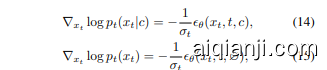

where $\sigma_{t}$ is the variance of the noise added to $x_{t}$ at timestep $t$ $\mathcal{Q}$ is the empty class, and $\epsilon_{\theta}(\cdot)$ is the diffusion model. Substituting Equations (14) and (15) into Equation (13) yields the score of posterior probability
其中 $\sigma_{t}$ 是在时间步 $t$ 添加到 $x_{t}$ 的噪声的方差,$\mathcal{Q}$ 是空类,$\epsilon_{\theta}(\cdot)$ 是扩散模型。将公式 (14) 和 (15) 代入公式 (13) 得到后验概率的得分

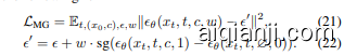
Then, our method applies the Bayes’ estimation in Equation (13) online and trains a conditional diffusion model to directly predict the score in Equation (12), instead of separately learning Equations (14) and (15) in the form of CFG. A straight-forward implementation is to adopt the objective in Equation (3) with a modified optimization target
随后,我们的方法在线应用了贝叶斯估计(见公式(13)),并训练了一个条件扩散模型来直接预测公式(12)中的得分,而不是以CFG的形式分别学习公式(14)和(15)。一个直接的实现是采用公式(3)中的目标,并修改优化目标
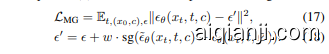
We apply the stop gradient operation, $\operatorname{sg}(\cdot)$ , which is a common practice of avoiding model collapse (Grill et al., 2020). We also use the Exponential Mean Average (EMA) counterpart of the online model, $\tilde{\epsilon}_{\theta}(\cdot)$ , to stabilize the training process and provide accurate estimations. For flow-based models, we have the similar objective
我们应用了停止梯度操作 $\operatorname{sg}(\cdot)$ ,这是避免模型崩溃的常见做法 (Grill et al., 2020)。我们还使用了在线模型的指数移动平均 (EMA) 版本 $\tilde{\epsilon}_{\theta}(\cdot)$ ,以稳定训练过程并提供准确的估计。对于基于流的模型,我们有类似的目标

where $u$ is the ground-truth fow in Equation (6)
其中 $u$ 是方程(6)中的真实流
During training, we randomly drop the condition $c$ in Equations (17) and (19) to $\mathcal{Q}$ with a ratio of $\lambda$ . These formulations transform the model itself into an implicit classifier and adjust the standard training objective of diffusion model in a self-supervised manner, allowing the joint optimization of generation quality and condition alignment with the minimum modification of existing pipelines.
在训练过程中,我们以比率 $\lambda$ 随机丢弃条件 $c$,将其从公式 (17) 和 (19) 中变化为 $\mathcal{Q}$。这些公式将模型本身转变为隐式分类器,并以自监督的方式调整扩散模型的标准训练目标,从而在最小化现有流程修改的情况下,实现对生成质量和条件对齐的联合优化。
3.3. Implementation Details
3.3. 实现细节
With the MG formulation in Equations (17) and (19), we have adequate options in the detailed implementations, such as incorporating an additional input of the guidance scale $w$ into networks, replacing the usage of empty class with the law of total probability, and whether to manual or automatically adjust the hyper-parameters.
通过方程 (17) 和 (19) 中的 MG 公式,我们在具体实现中有多种选择,例如将引导尺度 $w$ 的额外输入引入网络,用全概率定律替换空类的使用,以及手动或自动调整超参数。
Scale-aware networks. Similar to other distillation-based methods (Frans et al., 2024), the guidance scale $w$ canbe fed into the network as an additional condition. When augmented with $w$ -input, our models offer flexible choices of the balance between image quality and sample diversity during inference time. Note that our models require only one forward per step for all values of $w$ , while standard CFG needs two forwards, e.g. , one with condition and one without condition. In particular, we sample guidance scale from an specified interval, and the loss function are modified into the following form
尺度感知网络
Removing the empty class. Another option is whether to perform multitask learning of both conditional and unconditional generation with the same model. In CFG, the estimator in Equation (11) requires to train an unconditional model. However, the multitask learning can distract and hinder model capability. Using the law of total probability
移除空类。另一个选项是是否使用同一模型进行条件生成和无条件生成的多任务学习。在 CFG 中,公式 (11) 的估计器需要训练一个无条件模型。然而,多任务学习可能会分散注意力并阻碍模型能力。使用全概率定律

where $N$ different labels are used to estimate the unconditional score, our models focus on the conditional prediction and avoid the introduction of additional empty class.
其中使用 $N$ 个不同的标签来估计无条件得分,我们的模型专注于条件预测,并避免引入额外的空类。
Automatic adjustment of the hyper-parameter $w$ . While the scale $w$ in Equations (18) and (20) plays an important role, it is tedious and costly to perform manual search during training. Therefore, we introduce an automatic scheme to adjust $w$ .We begin with $w;=;0$ that corresponds to vanilla diffusion models, then update the value with EMA according to intermediate evaluation results. The value of $w$ is raised when quality decreases and suppressed otherwise, leading to an optimums when the training converged.
超参数 $w$ 的自动调整。虽然方程 (18) 和 (20) 中的尺度 $w$ 起着重要作用,但在训练过程中进行手动搜索既繁琐又成本高昂。因此,我们引入了一种自动调整 $w$ 的方案。我们首先从 $w;=;0$ 开始,这对应于普通的扩散模型,然后根据中间评估结果使用指数移动平均 (EMA) 更新 $w$ 的值。当质量下降时,$w$ 的值会提高,反之则会降低,从而在训练收敛时达到最优值。
4. Experiment
4. 实验
We first present a system-level comparison with state-of-theart models on ImageNet $256\times256$ conditional generation Then we conduct ablation experiments to investigate the detained designs of our method. Especially, we emphasize on the following questions:
我们首先在 ImageNet $256\times256$ 条件生成任务上与最先进的模型进行系统级比较,然后通过消融实验研究我们方法的详细设计。特别地,我们重点关注以下问题:
· How far can MG push the performances of existing diffusion models? (Tables 1 and 2, Section 4.2) · How does implementation details infuence the gain of proposed method? (Tables 3 to 6, Section 4.3) · Can MG scales to larger models and datasets with efficiency? (Tables 7 and 8, Figures 4 to 6, Section 4.3)
· MG 能在多大程度上提升现有扩散模型的性能?(表 1 和表 2,第 4.2 节)
· 实现细节如何影响所提出方法的增益?(表 3 到表 6,第 4.3 节)
· MG 能否高效扩展到更大的模型和数据集?(表 7 和表 8,图 4 到图 6,第 4.3 节)
Table 1: Experiments on ImageNet 256 without CFG. By deploying our method, the performances of both DiT-XL/2 and SiT-XL/2 are greatly boosted, achieving state-of-the-art.
表 1: 不带 CFG 的 ImageNet 256 实验结果。通过部署我们的方法,DiT-XL/2 和 SiT-XL/2 的性能都得到了显著提升,达到了最先进水平。
Table 2: Experiments on ImageNet 256 with CFG. Comparing to models with CFG, our method still obtains excellent results and surpasses others without efficiency loss.
4.1. Setup
4.1. 设置
Implementation and dataset. We follow the experiment pipelines in DiT (Peebles & Xie, 2023) and SiT (Ma et al., 2024). We use ImageNet (Deng et al., 2009; Russ a kov sky et al., 2015) dataset and the Stable Diffusion (Rombach et al., 2022) VAE to encode $256\times256$ images into the latent space of $\mathbb{R}^{32\times32\times4}$ . We conduct ablation experiments with the $\scriptstyle\mathrm{B}/2$ variant of DiT and SiT models and train for 400K iterations. During training, we use AdamW (Kingma, 2014; Loshchilov, 2019) optimizer and a batch size of 256 in consistent with DiT (Peebles & Xie, 2023) and SiT (Ma et al., 2024) for fair comparisons. For inference, we use 1000 sampling steps for DiT models and Euler-Maruyama sampler with 250 steps for SiT.
实现与数据集。我们遵循 DiT (Peebles & Xie, 2023) 和 SiT (Ma et al., 2024) 的实验流程。我们使用 ImageNet (Deng et al., 2009; Russakovsky et al., 2015) 数据集和 Stable Diffusion (Rombach et al., 2022) VAE 将 $256\times256$ 图像编码到 $\mathbb{R}^{32\times32\times4}$ 的潜在空间中。我们使用 DiT 和 SiT 模型的 $\scriptstyle\mathrm{B}/2$ 变体进行消融实验,并训练 400K 次迭代。在训练过程中,我们使用 AdamW (Kingma, 2014; Loshchilov, 2019) 优化器,并保持与 DiT (Peebles & Xie, 2023) 和 SiT (Ma et al., 2024) 一致的批量大小 256,以确保公平比较。在推理过程中,我们对 DiT 模型使用 1000 次采样步骤,对 SiT 使用 Euler-Maruyama 采样器,采样步骤为 250。
Baseline Models. We compare with several state-of-theart image generation models, including both diffusionbased and AR-based methods, which can be classified into the following three classes: (a) Pixel-space diffusion:
基线模型。我们与几种最先进的图像生成模型进行了比较,包括基于扩散和基于自回归(AR)的方法,这些模型可以分为以下三类:(a) 像素空间扩散:
Table 3: Experiments on scale w Diffusion Models without Classifier-Free Guidance
Table 4: Experiments on drop ratio $\lambda$
表 4: 丢弃率 $\lambda$ 实验
| MODEL | 入 | FID↓ | sFID↓ | IS↑ | PRE.↑ | REC.↑ |
|---|---|---|---|---|---|---|
| D1T-B/2 | 1.00 | 43.5 | 36.7 | 39.23 | 0.62 | 0.34 |
| +MG(ours) | 0.05 | 11.7 | 9.90 | 156.7 | 0.78 | 0.33 |
| +MG(ours) | 0.10 | 7.24 | 5.56 | 189.2 | 0.84 | 0.38 |
| +MG(ours) | 0.15 | 7.62 | 5.99 | 183.4 | 0.83 | 0.38 |
| +MG(ours) | 0.20 | 9.01 | 7.04 | 171.7 | 0.81 | 0.36 |
| SIT-B/2 | 1.00 | 33.0 | 27.8 | 65.24 | 0.68 | 0.35 |
| +MG(ours) | 0.05 | 10.8 | 9.25 | 168.8 | 0.80 | 0.34 |
| +MG(ours) | 0.10 | 6.49 | 5.69 | 212.3 | 0.86 | 0.38 |
| +MG(ours) | 0.15 | 6.77 | 5.89 | 207.4 | 0.85 | 0.37 |
| +MG(ours) | 0.20 | 8.87 | 8.06 | 199.6 | 0.84 | 0.37 |
ADM (Dhariwal & Nichol, 2021), $\mathrm{VDM++}$ (Kingma & Gao, 2023); (b) Latent-space diffusion: LDM (Rombach et al., 2022), U-ViT (Ba0 et al., 2023), MDTv2 (Ga0 et al., 2023), REPA (Yu et al., 2024b), Lightning D iT(L-DiT) (Yao & Wang, 2025), DiT (Peebles & Xie, 2023), SiT (Ma et al., 2024); (c) Auto-regressive models: VAR (Tian et al., 2024), RAR (Yu et al., 2024a), MAR (Li et al., 2024). These models consist of strong baselines and demonstrate the advantages of our method. Although our method does not requires CFG during inference, we still compare with these baselines under two settings, with and without CFG, for thoroughly investigations.
ADM (Dhariwal & Nichol, 2021), $\mathrm{VDM++}$ (Kingma & Gao, 2023); (b) 潜在空间扩散:LDM (Rombach et al., 2022), U-ViT (Ba0 et al., 2023), MDTv2 (Ga0 et al., 2023), REPA (Yu et al., 2024b), Lightning D iT(L-DiT) (Yao & Wang, 2025), DiT (Peebles & Xie, 2023), SiT (Ma et al., 2024); (c) 自回归模型:VAR (Tian et al., 2024), RAR (Yu et al., 2024a), MAR (Li et al., 2024)。这些模型构成了强大的基线,并展示了我们方法的优势。尽管我们的方法在推理过程中不需要CFG,但我们仍然在有和没有CFG的两种设置下与这些基线进行比较,以便进行彻底的研究。
Evaluation metrics. We report the commonly used Frechet inception distance (Heusel et al., 2017) with 50,000 samples (FID-50K). In addition, we report sFID (Nash et al., 2021), Inception Score (IS) (Salimans et al., 2016), Precision (Pre.), and Recall (Rec.) (Ky nk a an niemi et al., 2019) as supplementary metrics. We also report the time to generate one sample of each model in seconds to measure the trade-off between generation quality and computation budget.
评估指标。我们报告了常用的 Frechet inception distance (Heusel et al., 2017) 使用 50,000 个样本 (FID-50K)。此外,我们还报告了 sFID (Nash et al., 2021)、Inception Score (IS) (Salimans et al., 2016)、Precision (Pre.) 和 Recall (Rec.) (Ky nk a an niemi et al., 2019) 作为补充指标。我们还报告了每个模型生成一个样本所需的时间(以秒为单位),以衡量生成质量和计算预算之间的权衡。
4.2. Overall Performances
4.2. 整体性能
First of all, we present a through system-level comparison with recent state-of-the-art image generation approaches on ImageNet $256\times256$ dataset in Tables 1 and 2. As shown in Table 1, both DiT-XL/2 and SiT-XL/2 models greatly benefit from our method, achieving the outstanding performance gain of $78.9%$ and $84.4%$ . It is worth mentioning that our models do not apply modern techniques in the inference process, including rejection sampling (Tian et al.,
首先,我们在表1和表2中与近期最先进的图像生成方法在ImageNet $256\times256$ 数据集上进行了全面的系统级比较。如表1所示,DiT-XL/2和SiT-XL/2模型均从我们的方法中受益匪浅,分别实现了 $78.9%$ 和 $84.4%$ 的显著性能提升。值得一提的是,我们的模型在推理过程中并未应用现代技术,包括拒绝采样 (Tian et al.,
Table 5: Experiments on Model input $w$
表 5: 模型输入 $w$ 的实验
| MODEL | W-IN | FID↓ | SFID↓ | IS↑ | PRE.↑ | REC.↑ |
|---|---|---|---|---|---|---|
| DIT-B/2 | 43.5 | 36.7 | 39.23 | 0.62 | 0.34 | |
| +MG(ours) | 7.24 | 5.56 | 189.2 | 0.84 | 0.38 | |
| +MG(ours) | 8.13 | 6.03 | 175.1 | 0.84 | 0.39 | |
| SIT-B/2 | 33.0 | 27.8 | 65.24 | 0.68 | 0.35 | |
| +MG(ours) | 6.49 | 5.69 | 212.3 | 0.86 | 0.38 | |
| +MG(ours) | 7.33 | 5.96 | 207.4 | 0.85 | 0.38 |
Table 6: Experiments on empty class $\mathcal{Q}$
表 6: 空类 $\mathcal{Q}$ 上的实验
| MODEL | O-CLS | FID↓ | SFID↓ | IS↑ | PRE.↑ | REC.↑ |
|---|---|---|---|---|---|---|
| D1T-B/2 | 43.5 | 36.7 | 39.23 | 0.62 | 0.34 | |
| +MG(ours) | 9.66 | 8.73 | 174.4 | 0.81 | 0.35 | |
| +MG(ours) | 7.24 | 5.56 | 189.2 | 0.84 | 0.38 | |
| SIT-B/2 | 33.0 | 27.8 | 65.24 | 0.68 | 0.35 | |
| +MG(ours) | x | 9.03 | 7.96 | 183.3 | 0.82 | 0.35 |
| +MG(ours) | 6.49 | 5.69 | 212.3 | 0.86 | 0.38 |
2024), classifier-free guidance (Ho et al., 2020) and guidance interval (Ky nk a an niemi et al., 2024). Compared to advanced methods, our models are light-weight, e.g. 675M in contrast to RAR-XXL with 1.5B and MAR-H with 943M parameters, and consume less computational resources, for example, Lightning D iT uses DiT-XL/1 to reduce patch size to $1\times1$ and needs $16\times$ computation in attention operations.
2024), 无分类器引导 (Ho et al., 2020) 和引导间隔 (Ky nk a an niemi et al., 2024)。与先进方法相比,我们的模型轻量级,例如 675M 参数,而 RAR-XXL 有 1.5B 参数,MAR-H 有 943M 参数,并且消耗更少的计算资源,例如,Lightning D iT 使用 DiT-XL/1 将 patch 大小减少到 $1\times1$,并在注意力操作中需要 $16\times$ 的计算。
To facilitate a fair evaluation, we also compare with other methods with Classifier-free guidance. While prevalent diffusion models significantly benefit and are indispensable from CFG, it introduces an additional forward without condition and doubles the computation consumption s. Also, it usually requires a careful search over the hyper-parameter of guidance scale to achieve the best trade-off between quality and diversity. In contrast, our models still surpass other CFG-assisted methods and run with only half of the generation time.
为了进行公平的评估,我们还与其他使用无分类器引导(Classifier-free guidance, CFG)的方法进行了比较。虽然流行的扩散模型显著受益于 CFG 并且不可或缺,但它引入了额外的无条件前向传播,使计算消耗翻倍。此外,通常需要仔细搜索引导尺度的超参数,以在质量和多样性之间实现最佳平衡。相比之下,我们的模型仍然优于其他 CFG 辅助方法,并且生成时间仅为一半。
Finally, we report the time consumption for each model to generate one sample in seconds. Comparing to other diffusion-based approaches facilitated with vanilla CFG, our method runs significantly faster and does not sacrifice inference speed for sampling quality.
最后,我们报告了每个模型生成一个样本的时间消耗(以秒为单位)。与使用普通 CFG (Class-Free Guidance) 的其他基于扩散模型的方法相比,我们的方法运行速度显著更快,并且不会为了采样质量而牺牲推理速度。
4.3. Ablation study
4.3. 消融研究
To thoroughly understand the designs and subsequent influences of our method, we conduct ablation experiments on the key components, including the hyper-parameter $w$ $\lambda$ choices, whether the model takes $w$ as input, and the role of empty class during training. Moreover, we assess the s cal ability of our method in terms of both model size and dataset difficulty.
为了深入理解我们方法的设计及其后续影响,我们对关键组成部分进行了消融实验,包括超参数 $w$ 和 $\lambda$ 的选择、模型是否将 $w$ 作为输入,以及训练过程中空类的作用。此外,我们还从模型大小和数据集难度两个方面评估了我们方法的可扩展性。
Hyper-parameter $w$ In Equations (18) and (20), the hyperparameter $w$ controls the scale of posterior probability and serves an important role akin to the guidance scale in CFG, which is sensitive to FID-score. We conduct ablation experiments on the hyper-parameter $w$ and report results in
超参数 $w$ 在公式 (18) 和 (20) 中,超参数 $w$ 控制后验概率的尺度,其作用类似于 CFG 中的指导尺度,对 FID 分数敏感。我们对超参数 $w$ 进行了消融实验,并在
Table 7: Experiments on Model size. Our method scales to models with different sizes.
表 7: 模型大小实验。我们的方法适用于不同大小的模型。
| MODEL | FID↓ | SFID↓ | IS↑ | PRE.↑ | REC.↑ |
|---|---|---|---|---|---|
| D1T-B/2 +MG(ours) | 43.5 | 36.7 | 39.23 | 0.62 | 0.34 |
| D1T-L/2 | 7.24 23.3 | 5.56 18.4 | 189.2 132.7 | 0.84 0.73 | 0.38 0.40 |
| +MG(ours) D1T-XL/2 | 5.43 | 4.66 | 236.3 | 0.83 | 0.44 |
| +MG(ours) | 19.5 3.37 | 15.6 4.73 | 163.5 257.2 | 0.79 0.84 | 0.46 0.51 |
| SIT-B/2 +MG(ours) | 33.0 6.49 | 27.8 5.69 | 65.24 212.3 | 0.68 0.86 | 0.35 0.38 |
| SIT-L/2 | 18.9 | 16.3 | 173.2 | 0.71 | 0.42 |
| +MG(ours) | 4.50 | 4.03 | 243.9 | 0.85 | 0.46 |
| S1T-XL/2 | |||||
| +MG(ours) | 17.3 2.89 | 13.9 3.12 | 192.1 261.0 | 0.78 0.85 | 0.50 0.54 |
Table 8: Experiments on ImageNet 512. Our method scales to high-resolution image datasets.
表 8: ImageNet 512 上的实验。我们的方法可以扩展到高分辨率图像数据集。
| 模型 | FID↓ | SFID↓ | IS↑ | PRE.↑ | REC.↑ |
|---|---|---|---|---|---|
| D1T-XL/2 | 3.04 | 5.02 | 240.8 | 0.84 | 0.54 |
| +MG(ours) | 2.78 | 4.86 | 257.2 | 0.83 | 0.58 |
| SIT-XL/2 | 2.62 | 4.18 | 252.2 | 0.84 | 0.57 |
| +MG(ours) | 2.24 | 4.03 | 276.9 | 0.86 | 0.60 |
Table 3, where $w=1$ refers to vanilla forms in DiT (Peebles & Xie, 2023) and SiT (Ma et al., 2024). It is shown that the choice of $w$ also acts as a crucial role and balances the trade-off between quality and diversity.
表 3: 其中 $w=1$ 指的是 DiT (Peebles & Xie, 2023) 和 SiT (Ma et al., 2024) 中的原始形式。结果表明,$w$ 的选择也起着至关重要的作用,并在质量和多样性之间平衡取舍。
To overcome the tiresome and costly search of $w$ during training, we propose an adaptive approach to automatically adjust $w$ , which achieves comparable performance with manual search. Meanwhile, we can further apply CFG to our models in Figure 4 to fexibly adjust between better quality and diversity during inference.
为了克服训练过程中繁琐且耗时的 $w$ 搜索,我们提出了一种自适应方法来自动调整 $w$,该方法在性能上与手动搜索相当。同时,我们还可以在图 4 中的模型上进一步应用 CFG,以在推理过程中灵活调整质量和多样性之间的平衡。
Hyper-parameter $\lambda$ The relative ratio to train conditional and unconditional models, $\lambda$ , is also important to our method. The unconditional model is usually trained by randomly dropping the condition and replacing with an additional empty label for part of training data. In Table 4, we conduct ablation experiments on the hyper-parameter $\lambda$ report the corresponding results. We find that $\lambda$ is less sensitive than $w$ , and $\lambda\in{0.10,0.15}$ offers satisfactory performances.
超参数 $\lambda$
Model input $w$ Despite the same loss formulation in the Equation (17), it is optional whether our model takes the scale $w$ as an additional input. In Table 5, the models with $w$ input slightly lag behind the counterparts without $w$ -input but still exceeding the vanilla DiT-B/2 and SiT-B/2 with CFG, demonstrating the superiority of our method.
模型输入 $w$ 尽管在公式 (17) 中损失函数的形式相同,但我们的模型是否将尺度 $w$ 作为额外输入是可选的。在表 5 中,输入 $w$ 的模型略逊于不输入 $w$ 的模型,但仍然超过了使用 CFG 的原始 DiT-B/2 和 SiT-B/2,证明了我们方法的优越性。
Emptyclass $\mathcal{Q}$ In Table 6, we conduct ablation experiments on the introduction of additional empty class. While removing the empty class in our method leads to worse estimation of posterior probability, the generation performances are still on par with the vanilla CFG. It can also be improved by better estimation with the law of total probability or a larger batch size.
表 6: 空类 $\mathcal{Q}$ 的消融实验

Figure 4: FID-50K and Inception Score results as the guidance scale increases during inference. Our method is compatible with and can be wrapped into vanilla CFG.
图 4: 推理过程中随着引导尺度增加,FID-50K 和 Inception Score 的结果。我们的方法与普通的 CFG 兼容,并且可以封装在其中。

Figure 5: FID-5K results during training. Our method is $\geq6.5\times$ faster and $\approx60%$ better than vanilla DiT and SiT, even surpassing the results of CFG.
图 5: 训练期间的 FID-5K 结果。我们的方法比 vanilla DiT 和 SiT 快了 $\geq6.5\times$,并且效果提升了 $\approx60%$,甚至超过了 CFG 的结果。

Figure 6: FID-50K vs. number of parameters and sampling flops of different models, where our models are highlighted.
图 6: 不同模型的 FID-50K 与参数量及采样浮点运算次数的对比,其中我们的模型被突出显示。
Efficiency One key advantage of our method is that it not only improves inference speed by avoiding the second network forward of CFG, but also accelerates the training and convergence of diffusion models. In Figure 5, our method obtains $\geq6.5\times$ convergence speed and $\approx60%$ performance gain. In Figure 6, we plot the number of network parameters and sampling compute in TFlops versus FID-5OK of concurrent methods. When comparing number of network parameters, our method comes with the lowest FID and a small model size. When comparing sampling computes, our method achieves state-of-the-art performances in parallel with Lightning D iT (Yao & Wang, 2025), while requires Only $\approx12%$ computational resources.
效率
我们方法的一个关键优势在于,它不仅通过避免 CFG 的第二次网络前向传播来提高推理速度,还加速了扩散模型的训练和收敛。在图 5 中,我们的方法实现了 $\geq6.5\times$ 的收敛速度和 $\approx60%$ 的性能提升。在图 6 中,我们绘制了同时期方法的网络参数量与 TFlops 采样计算量相对于 FID-5OK 的对比图。在比较网络参数量时,我们的方法以最小的 FID 和较小的模型尺寸脱颖而出。在比较采样计算量时,我们的方法与 Lightning D iT (Yao & Wang, 2025) 并行实现了最先进的性能,而仅需 $\approx12%$ 的计算资源。

Figure 7: Uncurated samples of SiT-XL/2+MG on ImageNet $256\times256$
图 7: ImageNet $256\times256$ 上 SiT-XL/2+MG 的未筛选样本

Figure 8: Uncurated samples of SiT-XL/2+MG on ImageNet $512\times512$
图 8: ImageNet $512\times512$ 上 SiT-XL/2+MG 的未筛选样本
S cal ability Finally, the s cal ability to larger model and dataset of our method is of imparable significance. In Table 7, we conduct ablation stuides on model size with B/2, $L/2$ and $\mathrm{XL}/2$ variants of DiT and SiT models. It is demonstrated that our method is capable to boost the performance of models with different sizes and designs. We scale to ImageNet $512\times512$ dataset to validate our method in handling difficult distributions in Table 8. As depicted, our method also offers improvements on high-resolution tasks.
可扩展性
5. Conclusion
5. 结论
This work addresses the limitations of the commonly used Classifier-free guidance (CFG) of diffusion models, and proposes Model-guidance (MG) as an efficient and advantageous replacement. We first investigate the mechanism of CFG and locate the source of performance gain as a joint optimization of posterior probability. Then, we transcend the idea into the training process of diffusion models and directly learn the score of the joint distribution, $\nabla\log\tilde{p}{\theta}(x{t}|c);=;\nabla\log p_{\theta}(x_{t}|c)p_{\theta}(c|x_{t})^{w}$ .Comprehensive experiments demonstrate that our method significantly boosts the generation performance without efficiency loss, scales to different models and datasets, and achieves stateof-the-art results on ImageNet $256!\times!256$ dataset. We believe that this work contributes to future diffusion models.
本研究针对扩散模型常用的无分类器引导(Classifier-free guidance, CFG)的局限性,提出了一种高效且更具优势的模型引导(Model-guidance, MG)作为替代方案。我们首先探讨了 CFG 的机制,并将其性能提升的根源定位为后验概率的联合优化。随后,我们将这一理念融入扩散模型的训练过程,直接学习联合分布的得分,$\nabla\log\tilde{p}{\theta}(x{t}|c);=;\nabla\log p_{\theta}(x_{t}|c)p_{\theta}(c|x_{t})^{w}$。全面的实验表明,我们的方法在不损失效率的情况下显著提升了生成性能,适用于不同的模型和数据集,并在 ImageNet $256!\times!256$ 数据集上取得了最先进的结果。我们相信,这项工作将为未来的扩散模型研究做出贡献。
Impact Statements
影响声明
This paper propose methods in association with generative methods. There might be potential negative social impacts, e.g. generating fake portraits, as the core contribution of our work is a new algorithm of generative modeling. As possible mitigation strategies, we will restrict the access to these models in the planned release of code and models. We also validate that current detectors can effectively determine our generation results about human portraits.
本文提出了与生成方法相关的方法。由于我们工作的核心贡献是一种新的生成建模算法,可能存在潜在的负面社会影响,例如生成虚假肖像。作为可能的缓解策略,我们将在计划发布的代码和模型中限制对这些模型的访问。我们还验证了当前的检测器可以有效地确定我们生成的人像结果。
References
参考文献
Albergo, M. S., Boffi, N. M., and Vanden-Eijnden, E. Stochastic interpol ants: A unifying framework for flows and diffusions. arXiv preprint arXiv:2303.08797, 2023.
Albergo, M. S., Boffi, N. M., and Vanden-Eijnden, E. 随机插值:流与扩散的统一框架. arXiv preprint arXiv:2303.08797, 2023.
Bao, F., Nie, S., Xue, K., Cao, Y., Li, C., Su, H., and Zhu, J. All are worth words: A vit backbone for diffusion models. In Proceedings of the IEEE/CVF conference on computer vision and pattern recognition, pp. 22669-22679, 2023.
Bao, F., Nie, S., Xue, K., Cao, Y., Li, C., Su, H., and Zhu, J. All are worth words: A vit backbone for diffusion models. In Proceedings of the IEEE/CVF conference on computer vision and pattern recognition, pp. 22669-22679, 2023.
Black-Forest-Labs. Flux.1 model family, 2024. URL https://black forest labs.ai/ announcing-black-forest-labs/.
Black-Forest-Labs. Flux.1 模型系列, 2024. URL https://blackforestlabs.ai/announcing-black-forest-labs/.
Blattmann, A., Rombach, R., Ling, H., Dockhorn, T., Kim, S. W., Fidler, S., and Kreis, K. Align your latents: Highresolution video synthesis with latent diffusion models. In Proceedings of theIEEE/CVF Conference on Computer Vision and Pattern Recognition, pp. 22563-22575, 2023.
Blattmann, A., Rombach, R., Ling, H., Dockhorn, T., Kim, S. W., Fidler, S., 和 Kreis, K. 对齐你的潜在空间:基于潜在扩散模型的高分辨率视频合成。在 IEEE/CVF 计算机视觉与模式识别会议论文集,第 22563-22575 页,2023 年。
Brock, A., Donahue, J., and Simonyan, K. Large scale gan training for high fidelity natural image synthesis. In International Conference on Learning Representations, 2019.
Brock, A., Donahue, J., 和 Simonyan, K. 用于高保真自然图像合成的大规模 GAN 训练。在国际学习表征会议上,2019。
Chen, J., Jincheng, Y., Chongjian, G., Yao, L., Xie, E., Wang, Z., Kwok, J., Luo, P., Lu, H., and Li, Z. Pixart-Q: Fast training of diffusion transformer for photo realistic text-to-image synthesis. In The Twelfth International Conference on Learning Representations, 2024.
陈杰, 金成, 高崇建, 姚磊, 谢恩, 王峥, 郭杰, 罗平, 陆宏, 李志. Pixart-Q: 用于逼真文本到图像合成的扩散Transformer快速训练. 在第十二届国际学习表征会议, 2024.
Deng, J., Dong, W., Socher, R., Li, L.-J., Li, K., and Fei-Fei, L. Imagenet: A large-scale hierarchical image database. In 2009 IEEE conference on computer vision and pattern recognition, pp. 248-255. Ieee, 2009.
Deng, J., Dong, W., Socher, R., Li, L.-J., Li, K., and Fei-Fei, L. Imagenet: 一个大规模分层图像数据库。在 2009 年 IEEE 计算机视觉与模式识别会议上,第 248-255 页。IEEE, 2009.
Dhariwal, P. and Nichol, A. Diffusion models beat gans on image synthesis. Advances in neural information processing systems, 34:8780-8794, 2021.
Dhariwal, P. 和 Nichol, A. 扩散模型在图像合成上击败了GAN。神经信息处理系统进展,34:8780-8794, 2021。
Frans, K., Hafner, D., Levine, S., and Abbeel, P. One step diffusion via shortcut models.arXiv preprint arXiv:2410.12557,2024.
Frans, K., Hafner, D., Levine, S., and Abbeel, P. 通过捷径模型的一步扩散。arXiv 预印本 arXiv:2410.12557, 2024。
Gao, S., Zhou, P., Cheng, M.-M., and Yan, S. Masked diffusion transformer is a strong image synthesizer. In
Gao, S., Zhou, P., Cheng, M.-M., and Yan, S. 掩码扩散Transformer是强大的图像合成器。
Proceedings of theIEEE/C VF International Conference on Computer Vision, pp. 23164-23173, 2023.
IEEE/CVF 国际计算机视觉大会论文集,第 23164-23173 页,2023 年。
Grill, J.-B., Strub, F., Altché, F., Tallec, C., Richemond, P., Buch at s kaya, E., Doersch, C., Avila Pires, B., Guo, Z., Gheshlaghi Azar, M., et al. Bootstrap your own latent-a new approach to self-supervised learning. Advances in neural information processing systems, 33:21271-21284, 2020.
Grill, J.-B., Strub, F., Altché, F., Tallec, C., Richemond, P., Buchatskaya, E., Doersch, C., Avila Pires, B., Guo, Z., Gheshlaghi Azar, M., 等. Bootstrap your own latent-a new approach to self-supervised learning. 神经信息处理系统进展, 33:21271-21284, 2020.
Gupta, A., Yu, L., Sohn, K., Gu, X., Hahn, M., Li, F.- F., Essa, I., Jiang, L., and Lezama, J. Photo realistic video generation with diffusion models. In European Conference on Computer Vision, pp. 393-411. Springer, 2025.
Gupta, A., Yu, L., Sohn, K., Gu, X., Hahn, M., Li, F.- F., Essa, I., Jiang, L., and Lezama, J. 使用扩散模型生成逼真视频。在欧洲计算机视觉会议 (European Conference on Computer Vision) 上,pp. 393-411. Springer, 2025.
Heusel, M., Ramsauer, H., Unter thin er, T., Nessler, B., and Hochreiter, S. Gans trained by a two time-scale update rule converge to a local nash equilibrium. Advances in neural information processing systems, 30, 2017.
Heusel, M., Ramsauer, H., Unterthiner, T., Nessler, B., 和 Hochreiter, S. Gans trained by a two time-scale update rule converge to a local nash equilibrium. Advances in neural information processing systems, 30, 2017.
Ho, J. and Salimans, T. Classifier-free diffusion guidance. In NeurIPS 2021 Workshop on Deep Generative Models and Downstream Applications,2021.
Ho, J. 和 Salimans, T. 无分类器扩散引导。在 NeurIPS 2021 深度学习生成模型及其下游应用研讨会,2021。
Ho, J., Jain, A., and Abbeel, P. Denoising diffusion proba- bilistic models. Advances in neural information processing systems, 33:6840-6851, 2020.
Ho, J., Jain, A., and Abbeel, P. 去噪扩散概率模型。神经信息处理系统进展,33:6840-6851,2020。
Ho, J., Salimans, T., Gritsenko, A., Chan, W., Norouzi, M., and Fleet, D. J. Video diffusion models. Advances in Neural Information Processing Systems, 35:8633-8646, 2022.
Ho, J., Salimans, T., Gritsenko, A., Chan, W., Norouzi, M., and Fleet, D. J. 视频扩散模型. 神经信息处理系统进展, 35:8633-8646, 2022.
Hoogeboom, E., Heek, J., and Salimans, T. simple diffu- sion: End-to-end diffusion for high resolution images. In International Conference on Machine Learning, pp. 13213-13232.PMLR, 2023.
Hoogeboom, E., Heek, J., and Salimans, T. 简单扩散:用于高分辨率图像的端到端扩散方法。在国际机器学习会议上,第13213-13232页。PMLR,2023。
Karras, T., Laine, S., and Aila, T.A style-based generator architecture for generative adversarial networks.2019 IEEE/CVF Conference on Computer Vision and Pattern Recognition (CVPR), pp. 4396-4405, 2018. URL https://api.semantic scholar. org/CorpusID:54482423.
Karras, T., Laine, S., and Aila, T. 基于风格的生成器架构用于生成对抗网络。2019 IEEE/CVF 计算机视觉与模式识别会议 (CVPR), pp. 4396-4405, 2018. URL https://api.semantic scholar. org/CorpusID:54482423.
Karras, T., Aittala, M., Aila, T., and Laine, S. Elucidating the design space of diffusion-based generative models. Advances in neural information processing systems, 35: 26565-26577,2022.
Karras, T., Aittala, M., Aila, T., 和 Laine, S. 扩散基生成模型的设计空间解析。神经信息处理系统进展,35: 26565-26577, 2022。
Karras, T., Aittala, M., Ky nk a an niemi, T., Lehtinen, J., Aila, T., and Laine, S. Guiding a diffusion model with a bad version of itself. Advances in neural information processing systems,2024.
Karras, T., Aittala, M., Ky nk a an niemi, T., Lehtinen, J., Aila, T., and Laine, S. 使用自身的不良版本引导扩散模型。神经信息处理系统进展, 2024。
Kingma, D. P. Adam: A method for stochastic optimization. arXiv preprint arXiv:1412.6980, 2014.
Kingma, D. P. Adam: 一种随机优化方法。arXiv 预印本 arXiv:1412.6980, 2014。
Nichol, A. Q., Dhariwal, P., Ramesh, A., Shyam, P., Mishkin, P., Mcgrew, B., Sutskever, I., and Chen, M. Glide: Towards photo realistic image generation and editing with text-guided diffusion models. In International Conference on Machine Learning, pp. 16784-16804. PMLR,2022.
Nichol, A. Q., Dhariwal, P., Ramesh, A., Shyam, P., Mishkin, P., Mcgrew, B., Sutskever, I., and Chen, M. Glide: 基于文本引导扩散模型的逼真图像生成与编辑。In International Conference on Machine Learning, pp. 16784-16804. PMLR,2022.
Peebles, W. and Xie, S. Scalable diffusion models with transformers. In Proceedings of the IEEE/CVF International Conference on Computer Vision, pp. 4195-4205, 2023.
Peebles, W. 和 Xie, S. 使用 Transformer 的可扩展扩散模型。在 IEEE/CVF 国际计算机视觉会议论文集 (Proceedings of the IEEE/CVF International Conference on Computer Vision) 中,第 4195-4205 页,2023 年。
Podell, D., English, Z., Lacey, K., Blattmann, A., Dockhorn, T., Muller, J., Penna, J., and Rombach, R. Sdxl: Improving latent diffusion models for high-resolution image synthesis. In The Twelfth International Conference on Learning Representations, 2024.
Podell, D., English, Z., Lacey, K., Blattmann, A., Dockhorn, T., Muller, J., Penna, J., 和 Rombach, R. Sdxl: 提升潜在扩散模型以用于高分辨率图像合成。在第十二届国际学习表征会议中, 2024.
Polyak, A., Zohar, A., Brown, A., Tjandra, A., Sinha, A., Lee, A., Vyas, A., Shi, B., Ma, C.-Y., Chuang, C.-Y., et al. Movie gen: A cast of media foundation models. arXiv preprint arXiv:2410.13720,2024.
Polyak, A., Zohar, A., Brown, A., Tjandra, A., Sinha, A., Lee, A., Vyas, A., Shi, B., Ma, C.-Y., Chuang, C.-Y., 等. Movie gen: 媒体基础模型的应用. arXiv 预印本 arXiv:2410.13720, 2024.
Rombach, R., Blattmann, A., Lorenz, D., Esser, P., and Ommer, B. High-resolution image synthesis with latent diffusion models. In Proceedings of the IEEE/CVF con- ference on computer vision and pattern recognition, pp. 10684-10695,2022.
Rombach, R., Blattmann, A., Lorenz, D., Esser, P., 和 Ommer, B. 基于潜在扩散模型的高分辨率图像合成. 在 IEEE/CVF 计算机视觉与模式识别会议论文集, pp. 10684-10695, 2022.
Russ a kov sky, O., Deng, J., Su, H., Krause, J., Satheesh, S., Ma, S., Huang, Z., Karpathy, A., Khosla, A., Bernstein, M., et al. Imagenet large scale visual recognition challenge. International journal of computer vision, 115: 211-252,2015.
Russakovsky, O., Deng, J., Su, H., Krause, J., Satheesh, S., Ma, S., Huang, Z., Karpathy, A., Khosla, A., Bernstein, M., 等. Imagenet 大规模视觉识别挑战. 国际计算机视觉杂志, 115: 211-252, 2015.
Saharia, C., Chan, W., Saxena, S., Li, L., Whang, J., Denton, E. L., G has emi pour, K., Gontijo Lopes, R., Karagol Ayan, B., Salimans, T., et al. Photo realistic text-to-image diffusion models with deep language understanding. Advances in neural information processing systems, 35: 36479-36494, 2022.
Saharia, C., Chan, W., Saxena, S., Li, L., Whang, J., Denton, E. L., Ghasemipour, K., Gontijo Lopes, R., Karagol Ayan, B., Salimans, T., 等. 具有深度语言理解能力的逼真文本到图像扩散模型. 神经信息处理系统进展, 35: 36479-36494, 2022.
Salimans, T., Goodfellow, I., Zaremba, W., Cheung, V., Radford, A., and Chen, X. Improved techniques for training gans. Advances in neural information processing systems, 29, 2016.
Salimans, T., Goodfellow, I., Zaremba, W., Cheung, V., Radford, A., and Chen, X. 改进训练 GAN 的技术。神经信息处理系统进展,29,2016。
Sauer, A., Schwarz, K., and Geiger, A. Stylegan-xl: Scaling stylegan to large diverse datasets. ACM SIGGRAPH 2022 Conference Proceedings, 2022. URL https://api.semantic scholar.org/ CorpusID:246441861.
Sauer, A., Schwarz, K., and Geiger, A. Stylegan-xl: 将 Stylegan 扩展到大型多样化数据集。ACM SIGGRAPH 2022 会议论文集, 2022. URL https://api.semantic scholar.org/ CorpusID:246441861.
Sauer, A., Boesel, F., Dockhorn, T., Blattmann, A., Esser, P., and Rombach, R. Fast high-resolution image synthesis with latent adversarial diffusion distillation. In SIGGRAPH Asia 2024 Conference Papers, pPp. 1-11, 2024.
Sauer, A., Boesel, F., Dockhorn, T., Blattmann, A., Esser, P., and Rombach, R. 快速高分辨率图像合成与潜在对抗扩散蒸馏。在 SIGGRAPH Asia 2024 会议论文中,第 1-11 页,2024。