STYLEGAN2: Analyzing and Improving the Image Quality of StyleGAN 分析和改善 StyleGAN 的图像质量

Tero Karras
Samuli Laine
Miika Aittala
Janne Hellsten
Jaakko Lehtinen
Timo Aila

校对： 丫丫是只小狐狸

＞　译者语：stylegan改进版

摘要

StyleGAN在数据驱动的无条件生成图像建模中达到了最先进的结果。我们将揭露和分析其出现一些特征伪影的原因，并提出模型架构和训练方法方面的改进以解决这些问题。特别需要注意的是，我们重新设计了生成器归一化方法，重新审视了渐进式增长架构，并对生成器施加了正则化，使得从潜在矢量到图像的映射中得到良好质量的图像。除了改善图像质量外，使用路径长度调节器还带来了额外的好处，即生成器变得非常容易反转。这使得可以可靠地检测图像是否由特定网络生成。我们进一步对生成器是如何充分应用输出分辨率，并如何确定网络容量问题进行了可视化，从而激励我们训练更大的模型，以进一步提高质量。总体而言，我们改进的模型在现有的分布式指标质量和感知的图像质量方面都刷新了无条件图像建模的最先进技术指标。

ABSTRACT

The style-based GAN architecture (StyleGAN) yields state-of-the-art results in data-driven unconditional generative image modeling. We expose and analyze several of its characteristic artifacts, and propose changes in both model architecture and training methods to address them. In particular, we redesign generator normalization, revisit progressive growing, and regularize the generator to encourage good conditioning in the mapping from latent vectors to images. In addition to improving image quality, this path length regularizer yields the additional benefit that the generator becomes significantly easier to invert. This makes it possible to reliably detect if an image is generated by a particular network. We furthermore visualize how well the generator utilizes its output resolution, and identify a capacity problem, motivating us to train larger models for additional quality improvements. Overall, our improved model redefines the state of the art in unconditional image modeling, both in terms of existing distribution quality metrics as well as perceived image quality.

1 介绍 INTRODUCTION

The resolution and quality of images produced by generative methods, especially generative adversarial networks (GAN) [15], are improving rapidly [23, 31, 5]. The current state-of-the-art method for high-resolution image synthesis is StyleGAN [24], which has been shown to work reliably on a variety of datasets. Our work focuses on fixing its characteristic artifacts and improving the result quality further.

The distinguishing feature of StyleGAN [24] is its unconventional generator architecture. Instead of feeding the input latent code z∈Z only to the beginning of a the network, the mapping network f first transforms it to an intermediate latent code w∈W. Affine transforms then produce styles that control the layers of the synthesis network g via adaptive instance normalization (AdaIN) [20, 9, 12, 8]. Additionally, stochastic variation is facilitated by providing additional random noise maps to the synthesis network. It has been demonstrated [24, 38] that this design allows the intermediate latent space W to be much less entangled than the input latent space Z. In this paper, we focus all analysis solely on W, as it is the relevant latent space from the synthesis network’s point of view.

通过生成方法，尤其是生成对抗网络（GAN）[15]生成的图像的分辨率和质量正在迅速提高[23，31，5]。目前，用于高分辨率图像合成的最新方法是 StyleGAN [24]，它已被证明可以在各种数据集上可靠地工作。我们的工作重点是修复其特征伪影，并进一步提高结果质量。StyleGAN [24]的显著特征是其非常规的生成器体系结构。映射网络 f 不再将 输入隐编码 ${\bf z}\in\mathcal{Z}$输入网络，而是将其转换为中间隐编码
${\bf w}\in\mathcal{W}$。然后仿射变换生成控制图层的样式，并通过自适应实例归一化（AdaIN）[20、9、12、8]参与合成网络 g 进行合成。 另外，通过向合成网络提供额外的随机噪声图来促进随机变化.[24，38]研究表明，这种设计能让中间隐空间 W 比输入隐空间 Z 的纠缠少得多。。在本文中，我们所有的分析都只集中在 W 上，因为从合成网络的视角看，它是相关的隐空间。。

Many observers have noticed characteristic artifacts in images generated by StyleGAN [3]. We identify two causes for these artifacts, and describe changes in architecture and training methods that eliminate them. First, we investigate the origin of common blob-like artifacts, and find that the generator creates them to circumvent a design flaw in its architecture. In Section 2, we redesign the normalization used in the generator, which removes the artifacts. Second, we analyze artifacts related to progressive growing [23] that has been highly successful in stabilizing high-resolution GAN training. We propose an alternative design that achieves the same goal — training starts by focusing on low-resolution images and then progressively shifts focus to higher and higher resolutions — without changing the network topology during training. This new design also allows us to reason about the effective resolution of the generated images, which turns out to be lower than expected, motivating a capacity increase (Section 4).

Quantitative analysis of the quality of images produced using generative methods continues to be a challenging topic. Fréchet inception distance (FID) [19] measures differences in the density of two distributions in the high-dimensional feature space of a InceptionV3 classifier [39]. Precision and Recall (P&R) [36, 27] provide additional visibility by explicitly quantifying the percentage of generated images that are similar to training data and the percentage of training data that can be generated, respectively. We use these metrics to quantify the improvements.

Both FID and P&R are based on classifier networks that have recently been shown to focus on textures rather than shapes [11], and consequently, the metrics do not accurately capture all aspects of image quality. We observe that the perceptual path length (PPL) metric [24], introduced as a method for estimating the quality of latent space interpolations, correlates with consistency and stability of shapes. Based on this, we regularize the synthesis network to favor smooth mappings (Section 3) and achieve a clear improvement in quality. To counter its computational expense, we also propose executing all regularizations less frequently, observing that this can be done without compromising effectiveness.

Finally, we find that projection of images to the latent space W works significantly better with the new, path-length regularized generator than with the original StyleGAN. This has practical importance since it allows us to tell reliably whether a given image was generated using a particular generator (Section 5).

Our implementation and trained models are available at https://github.com/NVlabs/stylegan2

许多观察者已经注意到由 StyleGAN [3]生成的图像中的特征伪影。我们确定了造成这些伪影的两个原因，并描述了从结构和训练方法上进行改进来消除这些伪影的方法。
首先，我们研究了常见的斑点状伪影的起源，并发现生成器创建它们是为了规避其体系结构中的设计缺陷。在第 2 节中，我们重新设计了生成器中使用的归一化，该归一化消除了伪影。
其次，我们分析出伪影[23]和高分辨率 GAN 训练中很成功的一个方法 progressive growing渐进式增长相关。 我们提出了一个无需在训练中修改网络拓扑结构就能实现同样目标的设计-即训练从关注低分辨率图像开始，然后逐渐将焦点转移到越来越高的分辨率。这种新设计还能推理所生成图像的有效分辨率，事实证明这个有效分辨率低于预期，说明相关研究还有进一步的提升空间。

使用基于生成方法产生的图像质量的定量分析仍然是一个具有挑战性的话题。Frechet 初始距离（FID）[19]测量了InceptionV3 分类器的高维特征空间中两个分布的密度差异[39]。精确度和召回率（P＆R）[36，27]生成的与训练数据相似的图像的百分比和可以生成的训练数据的百分比，提供了额外的可见性。我们使用这些指标来量化stylegan2的改进。FID 和 P＆R 均基于分类器网络，最近已证明该分类器网络侧重于纹理而不是形状[11]，因此，这些度量不能准确地捕获图像质量的所有方面。我们观察到感知路径长度（PPL）度量[24]被引入作为一种估计潜在空间插值质量的方法，与形状的一致性和稳定性相关。在此基础上，我们对合成网络进行了正则化处理，以支持平滑映射（第 3 节），并明显实现了质量的提高。为了抵消其计算代价，我们建议不要么频繁地执行所有正则化，实验表明，这种做法其实对效果没什么影响。最后，我们发现，使用新的路径长度正则化生成器比使用原始 StyleGAN，将图像投影到潜在空间 W 的效果明显更好。这具有实际意义，因为这让我们可以可靠地辨别给定图像是否是用特定的生成器生成的。（第 5 节）。

我们的实施和经过训练的模型可在下方地址获得：https://github.com/NVlabs/stylegan2

2 消除因归一化导致的伪影 REMOVING NORMALIZATION ARTIFACTS

We begin by observing that most images generated by StyleGAN exhibit characteristic blob-shaped artifacts that resemble water droplets. As shown in Figure 1, even when the droplet may not be obvious in the final image, it is present in the intermediate feature maps of the generator The anomaly starts to appear around 64×64 resolution, is present in all feature maps, and becomes progressively stronger at higher resolutions. The existence of such a consistent artifact is puzzling, as the discriminator should be able to detect it.

We pinpoint the problem to the AdaIN operation that normalizes the mean and variance of each feature map separately, thereby potentially destroying any information found in the magnitudes of the features relative to each other. We hypothesize that the droplet artifact is a result of the generator intentionally sneaking signal strength information past instance normalization: by creating a strong, localized spike that dominates the statistics, the generator can effectively scale the signal as it likes elsewhere. Our hypothesis is supported by the finding that when the normalization step is removed from the generator, as detailed below, the droplet artifacts disappear completely.

我们首先观察到 StyleGAN 生成的大多数图像都呈现出类似于水滴的特征性斑点状伪影。如图 1 所示，即使水滴状伪影在最终图像中可能不明显，它也会出现在生成器的中间特征图中（见底部 1）。异常开始出现在 64×64 分辨率附近，并出现在所有特征图中，并且在更高的分辨率下变得越来越强。这种持续出现的伪影令人困惑，因为判别器应该能够检测到它。

我们将问题精确定位到 AdaIN 运算中，该运算分别归一化每个特征图的均值和方差，潜在地破坏在相关特征这个量级的一些信息。我们假设液滴伪影是生成器故意将信号强度信息偷偷经过实例归一化的结果：通过创建主导统计数据的强的局部尖峰，生成器可以有效地像在其它地方一样扩展该信号。研究者发现，：当从生成器中移除归一化步骤时，如下所述，水滴状伪影会完全消失。

图 1.实例归一化导致 StyleGAN 图像中出现类似水滴的伪影。这些在生成的图像中并不总是很明显，但是如果我们查看生成器网络内部的激活层，则问题始终存在，在所有从 64x64 分辨率开始的特征图中。这是困扰所有 StyleGAN 图像的系统性问题。

2.1. 生成器架构修正 GENERATOR ARCHITECTURE REVISITED

We will first revise several details of the StyleGAN generator to better facilitate our redesigned normalization. These changes have either a neutral or small positive effect on their own in terms of quality metrics.

Figure 2a shows the original StyleGAN synthesis network g [24], and in Figure 2b we expand the diagram to full detail by showing the weights and biases and breaking the AdaIN operation to its two constituent parts: normalization and modulation. This allows us to re-draw the conceptual gray boxes so that each box indicates the part of the network where one style is active (i.e., “style block”). Interestingly, the original StyleGAN applies bias and noise within the style block, causing their relative impact to be inversely proportional to the current style’s magnitudes. We observe that more predictable results are obtained by moving these operations outside the style block, where they operate on normalized data. Furthermore, we notice that after this change it is sufficient for the normalization and modulation to operate on the standard deviation alone (i.e., the mean is not needed). The application of bias, noise, and normalization to the constant input can also be safely removed without observable drawbacks. This variant is shown in Figure 2c, and serves as a starting point for our redesigned normalization.

我们将首先修改 StyleGAN 生成器的几个细节，以更好地促进我们重新设计归一化。就质量指标而言，这些变化本身产生中性或小小的积极影响。

图 2a 显示了原始的 StyleGAN 合成网络 g [24]，在图2b 中，我们将这张结构图的权重和偏差都展示出来，并将 AdaIN 操作分解为其两个组成部分：归一化和调制。这使我们可以重新绘制概念上的灰色框，以便每个框都指示网络中样式激活的部分（即“样式块”style block）。有趣的是，原始的 StyleGAN 在样式块内施加了偏置和噪音，使它们的相对影响与当前样式的大小成反比。
我们观察到，通过将这些操作移到style block之外（它们在未标准化的数据上进行操作），可以获得更可预测的结果。此外，我们注意到，在此更改之后，仅对标准偏差进行标准化和调制就足够了（即不需要均值）。对恒定输入应用的偏置，噪声和归一化也可以安全地消除，而没有明显的缺点。此变体如图 2c 所示，并作为我们重新设计的归一化的起点。

图 2.我们重新设计了 StyleGAN 合成网络的架构。（a）原始 StyleGAN，其中 A 表示从 W 学习的仿射变换，产生样式向量，而 B 表示噪声广播操作。（b）完整细节相同的图。在这里，我们将 AdaIN 分解为显式归一化后再进行调制，然后对每个特征图的均值和标准差进行操作。我们还对学习的权重（w），偏差（b）和常数输入（c）进行了注释，并重新绘制了灰色框，以便每个框都激活一种样式。激活函数（Leaky ReLU）总是在添加偏置后立即应用。（c）我们对原始架构进行了一些改动，这些改动在正文中是有效的。我们从一开始就删除了一些多余的操作，将 b 和 B 的相加移到样式的有效区域之外，并仅调整每个要素图的标准偏差。（d）修改后的体系结构使我们能够用“解调”操作代替实例归一化，该操作适用于与每个卷积层相关的权重。

2.2. 实例归一化修正 ### INSTANCE NORMALIZATION REVISITED

Given that instance normalization appears to be too strong, how can we relax it while retaining the scale-specific effects of the styles? We rule out batch normalization [21] as it is incompatible with the small minibatches required for high-resolution synthesis. Alternatively, we could simply remove the normalization. While actually improving FID slightly [27], this makes the effects of the styles cumulative rather than scale-specific, essentially losing the controllability offered by StyleGAN (see video). We will now propose an alternative that removes the artifacts while retaining controllability. The main idea is to base normalization on the expected statistics of the incoming feature maps, but without explicit forcing.

Recall that a style block in Figure 2c consists of modulation, convolution, and normalization. Let us start by considering the effect of a modulation followed by a convolution. The modulation scales each input feature map of the convolution based on the incoming style, which can alternatively be implemented by scaling the convolution weights:

鉴于实例归一化似乎过于强大，我们如何在保留样式特定比例的效果的同时减弱它呢？我们排除了批量归一化[21]，因为它与高分辨率合成所需的小型minibatch不兼容。或者，我们可以简单地删除归一化。尽管实际上稍微改善了FID [27]，但这使样式的效果得以累积而不是特定于比例，从而实质上失去了 StyleGAN 提供的可控制性（请参见视频）。现在，我们将提出一种替代方法，该方法在保留可控制性的同时删除了伪影。主要思想是基于传入特征图的预期统计量进行归一化，不显式强制。回想一下，图 2c 中的样式块由调制，卷积和归一化组成。让我们开始考虑卷积后的调制效果。调制根据输入样式缩放卷积的每个输入特征图，也可以通过缩放卷积权重来实现：
$$w'{ijk} = s_i \cdot w{ijk}$$

where w and w′ are the original and modulated weights, respectively, si is the scale corresponding to the ith input feature map, and j and k enumerate the output feature maps and spatial footprint of the convolution, respectively.

Now, the purpose of instance normalization is to essentially remove the effect of s from the statistics of the convolution’s output feature maps. We observe that this goal can be achieved more directly. Let us assume that the input activations are i.i.d. random variables with unit standard deviation. After modulation and convolution, the output activations have standard deviation of

其中 w 和 $w^{\prime}$分别是原始权重和调制权重，$s_i$ 是与第i 个输入特征图相对应的比例，而 j 和 k 分别列举输出特征图和卷积的空间下标。现在，实例归一化的目的是从卷积输出特征图的统计信息中实质上消除 s 的影响。我们观察到可以更直接地实现这一目标。让我们假设输入激活是独立同分布,带有单位标准偏差的随机变量。经过调制和卷积后，输出激活的标准偏差为$\sigma_{j}=\sqrt{{\sum{}}{w^{\prime}_{ijk}}^{2}}\tag 2$

i.e., the outputs are scaled by the L2 norm of the corresponding weights. The subsequent normalization aims to restore the outputs back to unit standard deviation. Based on Equation 2, this is achieved if we scale (“demodulate”) each output feature map j by 1/σj. Alternatively, we can again bake this into the convolution weights:

即，通过相应权重的 L2 范数来缩放输出。随后的标准化旨在将输出恢复为单位标准偏差。基于等式 2，如果我们将每个输出特征图 j 缩放（“解调”） ，则可以实现此目的。 或者，我们可以再次将其嵌入到卷积权重中:
$$
\begin{equation}
w''{ijk} = w'{ijk} \bigg/ \sqrt{\raisebox{0mm}[4.0mm][2.5mm]{\underset{i,k}{{}\displaystyle\sum{}}} {w'_{ijk}}^2 + \epsilon},
\label{eq:demodulation}
\end{equation}
$$

is a small constant to avoid numerical issues.

其中ϵ是避免数值问题的小常数。

We have now baked the entire style block to a single convolution layer whose weights are adjusted based on s using Equations 1 and 3 (Figure 2d). Compared to instance normalization, our demodulation technique is weaker because it is based on statistical assumptions about the signal instead of actual contents of the feature maps. Similar statistical analysis has been extensively used in modern network initializers [13, 18], but we are not aware of it being previously used as a replacement for data-dependent normalization. Our demodulation is also related to weight normalization [37] that performs the same calculation as a part of reparameterizing the weight tensor. Prior work has identified weight normalization as beneficial in the context of GAN training [42].

Our new design removes the characteristic artifacts (Figure 3) while retaining full controllability, as demonstrated in the accompanying video. FID remains largely unaffected (Table 1, rows a, b), but there is a notable shift from precision to recall. We argue that this is generally desirable, since recall can be traded into precision via truncation, whereas the opposite is not true [27]. In practice our design can be implemented efficiently using grouped convolutions, as detailed in Appendix B. To avoid having to account for the activation function in Equation 3, we scale our activation functions so that they retain the expected signal variance.

现在，我们已经将整个样式块嵌入到单个卷积层，其权重使用公式 1 和 3 基于 s 进行调整（图 2d）。与实例归一化相比，我们的解调技术较弱，因为它基于信号的统计假设，而不是特征图的实际内容。类似的统计分析已在现代网络初始化程序中广泛使用[13，18]，但我们不知道它先前已被用来代替依赖数据的归一化。我们的解调也与权重归一化[37]有关，权重归一化[37]执行与重新设定权重张量相同的计算。先前的工作已经证明权重归一化在 GAN 训练中是有益的[42]。我们的新设计消除了特征伪影（图 3），同时保持了完全的可控制性，如随附视频所示。FID 基本上不受影响（表1，行 A，B），但是从 Precision 到 Recall 有着明显的转变。我们认为这通常是合乎需要的，因为可以通过截断将召回率转换为精度，但事实并非如此[27]。实际上，我们的设计可以是如附录 B 所述，使用分组卷积有效地实现该功能。为避免必须在公式 3 中考虑激活函数，我们对激活函数进行缩放，以使其保留预期的信号方差。

图 3.用解调代替归一化可从图像和激活中删除特征伪像。

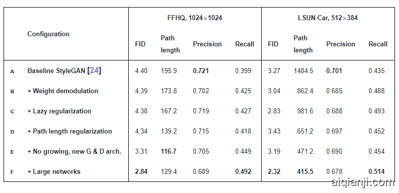
表 1：主要结果。对于每次训练过程，这里选出的都是 FID 最低的训练快照。研究者使用不同的随机种子计算了每个指标 10 次，并报告了平均结果。「path length」一列对应于 PPL 指标，这是基于 W 中的路径端点（path endpoints）而计算得到的。对于 LSUN 数据集，报告的路径长度是原本为 FFHQ 提出的无中心裁剪的结果。FFHQ 数据集包含 7 万张图像，研究者在训练阶段向判别器展示了 2500 万张图像。对于 LSUN CAR 数据集，对应的数字是 89.3 万和 5700 万。

3. 图像质量和生成器平滑度 IMAGE QUALITY AND GENERATOR SMOOTHNESS

While GAN metrics such as FID or Precision and Recall (P&R) successfully capture many aspects of the generator, they continue to have somewhat of a blind spot for image quality. For an example, refer to Figures 13 and 14 that contrast generators with identical FID and P&R scores but markedly different overall quality.

尽管 GAN 度量标准（例如 FID(Frechet inception distance) 或 Precision and Recall（P＆R））成功地捕获了生成器的许多方面，但它们仍然在图像质量上处于盲点。例如，请参考图 13 和图 14，它们对比了具有相同 FID 和 P＆R 分数但整体质量明显不同的生成器。 （我们认为，明显的不一致的关键在于要素空间的特定选择，而不是 FID 或 P＆R 的基础。最近发现，使用 ImageNet [35]训练的分类器倾向于将决策更多地基于纹理而不是形状[11]，而人类则强烈关注形状[28]。这是有意义的，因为 FID 和 P＆R 使用分别来自 InceptionV3 [39]和 VGG-16 [39]的高级特征，这些特征是通过这种方式进行训练的，因此可以预期偏向于纹理检测。这样，具有强烈的猫的纹理的图像可能看起来彼此更相似，比人类观察者所在意的细节还要强，从而部分损害了基于密度的度量（FID）和多方面的覆盖度量（P＆R）。）

We observe an interesting correlation between perceived image quality and perceptual path length (PPL) [24], a metric that was originally introduced for quantifying the smoothness of the mapping from a latent space to the output image by measuring average LPIPS distances [49] between generated images under small perturbations in latent space. Again consulting Figures 13 and 14, a smaller PPL (smoother generator mapping) appears to correlate with higher overall image quality, whereas other metrics are blind to the change. Figure 4 examines this correlation more closely through per-image PPL scores computed by sampling latent space around individual points in W on StyleGAN trained on LSUN Cat: low PPL scores are indeed indicative of high-quality images, and vice versa. Figure 5a shows the corresponding histogram of per-image PPL scores and reveals the long tail of the distribution. The overall PPL for the model is simply the expected value of the per-image PPL scores.

It is not immediately obvious why a low PPL should correlate with image quality. We hypothesize that during training, as the discriminator penalizes broken images, the most direct way for the generator to improve is to effectively stretch the region of latent space that yields good images. This would lead to the low-quality images being squeezed into small latent space regions of rapid change. While this improves the average output quality in the short term, the accumulating distortions impair the training dynamics and consequently the final image quality.

我们观察到了感知的图像质量和感知路径长度（PPL）之间的有趣关系[24]，该指标最初是通过测量在隐空间中的小扰动下生成的图像之间的平均 LPIPS 距离来量化从隐空间到输出图像的映射平滑度的指标[49]。再次参考图 13 和14，较小的PPL（平滑的生成器映射）似乎与较高的整体图像质量相关，而其他指标则看不到该变化。 图 4 证明这种相关性更强，通过在 LSUN CAT 上训练的 StyleGAN 上的 W 上各个点周围的潜在空间采样得出的每幅图像 PPL 分数可以了解到：PPL 分数低实际上表示图像的质量高，反之亦然。

图 4.使用基线 StyleGAN（表 1 中的配置 A）在感知路径长度和图像质量之间建立联系。（a）PPL 低（≤第 10 个百分点）的随机例子。（b）PPL 高（≥第 90 个百分点）的示例。 PPL 分数与图像的语义一致性之间存在明显的相关性。

图 5a 显示了每个图像 PPL 得分的相应直方图，并揭示了分布的长尾。该模型的总体 PPL 只是每个图像 PPL 得分的预期值。为何 PPL 值低与图像质量的关联不太明显？我们假设在训练过程中，由于判别器会对残破的图像进行惩罚，因此生成器改进的最直接方法是有效地拉伸产生良好图像的潜在空间区域，这将导致劣质图像被压缩进快速变化的小型隐藏空间。虽然这可以在短期内提高平均输出质量，但累积的失真会损害训练状态，进而由此影响最终的图像质量。

This empirical correlation suggests that favoring a smooth generator mapping by encouraging low PPL during training may improve image quality, which we show to be the case below. As the resulting regularization term is somewhat expensive to compute, we first describe a general optimization that applies to all regularization techniques.

这种经验相关性表明，在训练过程中通过鼓励低 PPL来支持平滑的生成器映射可能会改善图像质量。实验表明，事实确实如此。由于所得到的正则化项在一定程度上计算成本较高，所以首先描述了一种可应用于所有正则化技术的通用优化方法。

3.1. 延迟正则化（Lazy regularization）

Typically the main loss function (e.g., logistic loss [15]) and regularization terms (e.g., R1 [30]) are written as a single expression and are thus optimized simultaneously. We observe that typically the regularization terms can be computed much less frequently than the main loss function, thus greatly diminishing their computational cost and the overall memory usage. Table 1, row c shows that no harm is caused when R1 regularization is performed only once every 16 minibatches, and we adopt the same strategy for our new regularizer as well. Appendix B gives implementation details.

通常，主要损失函数（例如，逻辑损失[15]）和正则化项（例如， [30]）被写为一个表达式，因此被同时优化。我们观察到，正规化项的计算频率通常比主要损失函数低得多，从而大大降低了它们的计算成本和整体内存使用量。表 1 中的 C 行显示，每 16 个小批量仅执行一次 正则化时，不会造成任何危害，并且我们对新的正则化器也采用了相同的策略。附录 B 给出了实现细节。

3.2. 路径长度正则化 PATH LENGTH REGULARIZATION

Excess path distortion in the generator is evident as poor local conditioning: any small region in W becomes arbitrarily squeezed and stretched as it is mapped by g. In line with earlier work [33], we consider a generator mapping from the latent space to image space to be well-conditioned if, at each point in latent space, small displacements yield changes of equal magnitude in image space regardless of the direction of perturbation.

At a single w∈W, the local metric scaling properties of the generator mapping g(w):W↦Y are captured by the Jacobian matrix Jw=∂g(w)/∂w. Motivated by the desire to preserve the expected lengths of vectors regardless of the direction, we formulate our regularizer as

生成器中的路径失真过大显然是不良的局部条件：W中的任何小区域在被 g 映射时都会被任意挤压和拉伸。与早期工作[33]一致，如果在潜在空间中的每个点处，小的位移都在图像空间中产生相同大小的变化，而与摄动方向无关，则我们认为从潜在空间到图像空间的生成器映射条件良好。在单个${\bf w}\in\mathcal{W}$处，生成器映射g $g({\bf w}):\mathcal{W}\mapsto\mathcal{Y}$ 的局部度量比例缩放属性由雅可比矩阵$\mathbf{J}_{\bf w}={\partial g({\bf w})}/{\partial{\bf w}}$捕获。出于保持向量预期长度（无论方向如何）的动机，我们将正则化定义为：

$$\mathbb{E}{{\bf w},{\bf y}\sim\mathcal{N}(0,\mathbf{I})}\left( \left\lVert\mathbf{J}{\bf w}^{T}{\bf y}\right\rVert_{2}-a \right)^{2} \tag 4$$

where y are random images with normally distributed pixel intensities, and w∼f(z), where z are normally distributed. We show in Appendix C that, in high dimensions, this prior is minimized when Jw is orthogonal (up to a global scale) at any w. An orthogonal matrix preserves lengths and introduces no squeezing along any dimension.

To avoid explicit computation of the Jacobian matrix, we use the identity ${\bf J}^{T}{\bf w}{\bf y}=\nabla{\bf w}(g({\bf w})\cdot{\bf y})$, which is efficiently computable using standard backpropagation [6]. The constant a is set dynamically during optimization as the long-running exponential moving average of the lengths $\lVert{\bf J}^{T}{\bf w}{\bf y}\rVert{2}$, allowing the optimization to find a suitable global scale by itself.

其中 y 是具有正态分布像素强度的随机图像，而${\bf w}\sim f(\mathbf{z})$，其中 z 是正态分布。我们在附录 C 中显示，在高维上，当 $J_w$在任何 w 处都是正交的（最大到全局范围）时，该先验会最小化。正交矩阵会保留长度，并且不会沿任何维度压缩。为了避免对雅可比矩阵的显式计算，我们使用恒等式${\bf J}^{T}{\bf w}{\bf y}=\nabla{\bf w}(g({\bf w})\cdot{\bf y})$，它可以使用标准反向传播有效地计算[6]。
常数 a 在优化过程中动态设置为长度$\lVert{\bf J}^{T}{\bf w}{\bf y}\rVert{2}$ 的长期指数移动平均值，从而使优化本身可以找到合适的全局标度。

Our regularizer is closely related to the Jacobian clamping regularizer presented by Odena et al. [33]. Practical differences include that we compute the products$\mathbf{J}_{\bf w}\boldsymbol{\delta}$analytically whereas they use finite differences for estimating Jwδ with Z∋δ∼N(0,I). It should be noted that spectral normalization [31] of the generator [45] only constrains the largest singular value, posing no constraints on the others and hence not necessarily leading to better conditioning.

In practice, we notice that path length regularization leads to more reliable and consistently behaving models, making architecture exploration easier. Figure 5b shows that path length regularization clearly improves the distribution of per-image PPL scores. Table 1, row d shows that regularization reduces PPL, as expected, but there is a tradeoff between FID and PPL in LSUN Car and other datasets that are less structured than FFHQ. Furthermore, we observe that a smoother generator is easier to invert (Section 5).

我们的正则化器与 Odena 等人提出的 Jacobian“夹紧”正则化器密切相关[33]。实际的差异包括我们通过分析计算出乘积$\mathbf{J}_{\bf w}\boldsymbol{\delta}$，而它们使用有限的差异来估计满足$\mathcal{Z}\ni\boldsymbol{\delta}\sim\mathcal{N}(0,\mathbf{I})$的 。应当指出，生成器[45]的频谱归一化[31]仅约束最大奇异值，对其他奇异值没有约束，因此不一定导致更好的调节。
在实践中，我们注意到路径长度正则化导致更可靠和始终如一的行为模型，从而使架构探索更加容易。图 5b 显示，路径长度正则化明显改善了每个图像 PPL 分数的分布。表 1 的 D 行表明，正则化可以按预期方式降低 PPL，但在 LSUN CAR 和结构比 FFHQ 少的其他数据集中，FID和 PPL 之间需要权衡。此外，我们观察到，更平滑的生成器更易于反转（第 5 节）。

4. 渐进式增长修正 PROGRESSIVE GROWING REVISITED

Progressive growing [23] has been very successful in stabilizing high-resolution image synthesis, but it causes its own characteristic artifacts. The key issue is that the progressively grown generator appears to have a strong location preference for details; the accompanying video shows that when features like teeth or eyes should move smoothly over the image, they may instead remain stuck in place before jumping to the next preferred location. Figure 6 shows a related artifact. We believe the problem is that in progressive growing each resolution serves momentarily as the output resolution, forcing it to generate maximal frequency details, which then leads to the trained network to have excessively high frequencies in the intermediate layers, compromising shift invariance [48]. Appendix A shows an example. These issues prompt us to search for an alternative formulation that would retain the benefits of progressive growing without the drawbacks.

渐进生长[23]在稳定高分辨率图像合成方面已经非常成功，但它会导致其自身的特征失真。关键问题在于，逐渐增长的生成器似乎对细节的位置偏好很高。
随附的视频显示当牙齿或眼睛等特征在图像上平滑移动时，它们可能会停留在原位，然后跳到下一个首选位置。图 6 显示了相关的伪像。我们认为问题在于，在逐步增长的过程中，每个分辨率都会瞬间用作输出分辨率，迫使其生成最大频率细节，然后导致受过训练的网络在中间层具有过高的频率，从而损害了位移不变性[48]。附录 A 显示了一个示例。这些问题促使我们寻找一种替代方法，该方法将保留渐进式增长的好处而消除弊端。

4.1. 可选的网络架构 ALTERNATIVE NETWORK ARCHITECTURES

While StyleGAN uses simple feedforward designs in the generator (synthesis network) and discriminator, there is a vast body of work dedicated to the study of better network architectures. In particular, skip connections [34, 22], residual networks [17, 16, 31], and hierarchical methods [7, 46, 47] have proven highly successful also in the context of generative methods. As such, we decided to re-evaluate the network design of StyleGAN and search for an architecture that produces high-quality images without progressive growing.

Figure 7a shows MSG-GAN [22], which connects the matching resolutions of the generator and discriminator using multiple skip connections. The MSG-GAN generator is modified to output a mipmap [41] instead of an image, and a similar representation is computed for each real image as well. In Figure 7b we simplify this design by upsampling and summing the contributions of RGB outputs corresponding to different resolutions. In the discriminator, we similarly provide the downsampled image to each resolution block of the discriminator. We use bilinear filtering in all up and downsampling operations. In Figure 7c we further modify the design to use residual connections.3 This design is similar to LAPGAN [7] without the per-resolution discriminators employed by Denton et al.

虽然 StyleGAN 在生成器（合成网络）和判别器中使用简单的前馈设计，但仍有大量工作致力于研究更好的网络体系结构。特别地，在生成方法的背景下，跳跃连接[34、22]，残差网络[17、16、31]和分层方法[7、46、47]也被证明是非常成功的。因此，我们决定重新评估 StyleGAN 的网络设计，并寻找一种能够生成高质量图像而不会逐渐增长的体系结构。图 7a 显示了 MSG-GAN [22]，它使用多个跳越连接来连接生成器和判别器的匹配分辨率。修改了 MSG-GAN 生成器以输出多维图像（mipmap） [41]而不是图像，并且还为每个真实图像计算了类似的表示形式。在图 7b 中，我们通过上采样并求和对应于不同分辨率的 RGB 输出的贡献来简化此设计。在判别器中我们类似地将下采样的图像提供给判别器的每个分辨率块。我们在所有上采样和下采样操作中都使用了双线性滤波。在图 7c 中，我们进一步修改了设计以使用残差连接（见底部3）。此设计类似于 LAPGAN [7]，但没有 Denton 等人使用的逐分辨率判别器。

图 7：三种生成器（虚线上面）和判别器架构。Up 和 Down 分别表示双线性的上采样和下采样。在残差网络中，这些也包含用于调整特征图数量的 1×1 卷积。tRGB 和 fRGB 可将每个像素的数据在 RGB 和高维数据之间转换。配置 E 和 F 所用的架构用绿色标注。

Table 2 compares three generator and three discriminator architectures: original feedforward networks as used in StyleGAN, skip connections, and residual networks, all trained without progressive growing. FID and PPL are provided for each of the 9 combinations. We can see two broad trends: skip connections in the generator drastically improve PPL in all configurations, and a residual discriminator network is clearly beneficial for FID. The latter is perhaps not surprising since the structure of discriminator resembles classifiers where residual architectures are known to be helpful. However, a residual architecture was harmful in the generator — the lone exception was FID in LSUN Car when both networks were residual.

For the rest of the paper we use a skip generator and a residual discriminator, and do not use progressive growing. This corresponds to configuration e in Table 1, and as can be seen table, switching to this setup significantly improves FID and PPL.

表 2 比较了三种生成器架构和三种判别器架构：
StyleGAN 中使用的原始前馈网络，跳越连接和残差网络，所有这些网络的训练都没有用渐进式增长(progressive growing)。表中为 9 种组合都计算了 FID 和 PPL。我们可以看到两个趋势：在所有配置中，生成器中的跳越连接会大大改善 PPL，而残差的判别器网络显然对 FID 有利。后者也许不足为奇，因为判别器的结构就是分类器（残差结构会对分类器有利）。但是，残差的体系结构对生成器有害。当两个网络都是残差的时，唯一的例外是 LSUN CAR 中的 FID。在本文的其余部分，我们使用跳越生成器skip generator和残差判别器，而不使用渐进式增长。这对应于表 1 中的配置 E，从表中可以看出，切换到该设置可以显著改善 FID 和 PPL。

4.2. 分辨率的使用 RESOLUTION USAGE

The key aspect of progressive growing, which we would like to preserve, is that the generator will initially focus on low-resolution features and then slowly shift its attention to finer details. The architectures in Figure 7 make it possible for the generator to first output low resolution images that are not affected by the higher-resolution layers in a significant way, and later shift the focus to the higher-resolution layers as the training proceeds. Since this is not enforced in any way, the generator will do it only if it is beneficial. To analyze the behavior in practice, we need to quantify how strongly the generator relies on particular resolutions over the course of training.

Since the skip generator (Figure 7b) forms the image by explicitly summing RGB values from multiple resolutions, we can estimate the relative importance of the corresponding layers by measuring how much they contribute to the final image. In Figure 8a, we plot the standard deviation of the pixel values produced by each tRGB layer as a function of training time. We calculate the standard deviations over 1024 random samples of w and normalize the values so that they sum to 100%.

对于渐进式增长，我们希望保留的的关键点是，生成器最初将关注低分辨率特性，然后慢慢将注意力转移到更精细的细节上。图7中的体系结构使得生成器可以首先输出不受高分辨率层影响的低分辨率图像，然后随着训练的进行将焦点转移到高分辨率层。因为这并不是强制执行的，所以只有在有益的情况下，生成器才会这样做。为了分析实际中的行为，我们需要量化生成器在训练过程中对特定解决方案的依赖程度。

由于跳转型生成器(图7b)通过显式地将多分辨率的 RGB 值相加形成图像，因此我们可以通过测量对应层对最终图像的贡献程度来估计它们的相对重要性。在图8a 中，我们绘制了每个 tRGB 层产生的像素值的标准差与训练时间的关系。我们计算了 w 的1024个随机样本的标准差，并将其归一化，保证总和为为100% 。

At the start of training, we can see that the new skip generator behaves similar to progressive growing — now achieved without changing the network topology. It would thus be reasonable to expect the highest resolution to dominate towards the end of the training. The plot, however, shows that this fails to happen in practice, which indicates that the generator may not be able to “fully utilize” the target resolution. To verify this, we inspected the generated images manually and noticed that they generally lack some of the pixel-level detail that is present in the training data — the images could be described as being sharpened versions of 512^2 images instead of true 1024^2 images.

This leads us to hypothesize that there is a capacity problem in our networks, which we test by doubling the number of feature maps in the highest-resolution layers of both networks.4(4We double the number of feature maps in resolutions 64^2–1024^2 while keeping other parts of the networks unchanged. This increases the total number of trainable parameters in the generator by 22% (25M → 30M) and in the discriminator by 21% (24M → 29M).） This brings the behavior more in line with expectations: Figure 8b shows a significant increase in the contribution of the highest-resolution layers, and Table 1, row f shows that FID and Recall improve markedly.

Table 3 compares StyleGAN and our improved variant in several LSUN categories, again showing clear improvements in FID and significant advances in PPL. It is possible that further increases in the size could provide additional benefits.

在训练开始时，我们可以看到新的跳转型生成器的行为类似于渐进式增长-无需更改网络拓扑即可实现。因此，期望最高分辨率在训练结束时占优势是合理的。但是，该图表明在实践中这没有发生，这表明生成器可能无法“完全利用”目标分辨率。为了验证这一点，我们手动检查了生成的图像，发现它们通常缺乏训练数据中存在的一些像素级细节-图像可以描述为512尺寸图像的锐化版本，而不是真实的1024图像。

这导致我们假设存在容量问题在我们的网络中，我们通过将两个网络的最高分辨率层中的特征图的数量加倍来进行测试（见底部 4）。这使行为更加符合预期：图 8b 显示了贡献的显著增加，表 1 的 F 行显示FID 和 Recall 显著提高。表 3 在几个 LSUN 类别中比较了 StyleGAN 和我们改进的变体，再次显示了 FID 的明显改进和 PPL 的显著进步。尺寸的进一步增加可能会带来更多好处。

图 8.每个分辨率对生成器输出的贡献与训练时间的关系。纵轴显示了不同分辨率的相对标准偏差的刻度值，横轴对应于训练进度，以判别器显示的数百万个训练图像进行测量。我们可以看到，网络一开始就专注于低分辨率图像，并且随着训练的进行逐渐将其注意力转移到更大的分辨率上。在（a）中，生成器基本上输出512的图像，并对其进行较小锐化产生1024的图像，而在（b）中，较大的网络更多地关注高分辨率细节。

这使我们假设，我们的网络存在容量问题，我们通过将两个网络的最高分辨率层的特征映射数量增加一倍来进行测试。这使生成器中的可训练参数总数增加了22% (25M →30M) ，判别器中的可训练参数总数增加了21% (24M →29M)。这使得行为更加符合预期: 图8b 显示了最高分辨率层贡献的显著增加，表1的 f 行显示 FID 和 Recall 显著改善。

表3比较了 StyleGAN 和我们在几个 LSUN 类别中的改进，再次显示了 FID 的明显改进和 PPL 的显著进步。规模的进一步扩大可能会带来额外的好处。

表 3.使用 FID 和 PPL 测量的 LSUN 数据集的改进。我们对 CAR 进行了 5700 万幅图像的训练，对 CAT 进行了 88M 的训练，对CHURCH 进行了 48M 的训练，对 HORSE 进行了 100M 的训练。

5. 将图像投影到潜在空间 PROJECTION OF IMAGES TO LATENT SPACE

Inverting the synthesis network g is an interesting problem that has many applications. Manipulating a given image in the latent feature space requires finding a matching latent vector w for it first. Also, as the image quality of GANs im-proves, it becomes more important to be able to attribute a potentially synthetic image to the network that generated it.

Previous research [1, 10] suggests that instead of finding a common latent vector w, the results improve if a separate w is chosen for each layer of the generator. The same approach was used in an early encoder implementation [32]. While extending the latent space in this fashion finds a closer match to a given image, it also enables projecting arbitrary images that should have no latent representation. Focusing on the forensic detection of generated images, we concentrate on finding latent codes in the original, unextended latent space, as these correspond to images that the generator could have produced.

Our projection method differs from previous methods in two ways. First, we add ramped-down noise to the latent code during optimization in order to explore the latent space more comprehensively. Second, we also optimize the stochastic noise inputs of the StyleGAN generator, regularizing them to ensure they do not end up carrying coherent signal. The regularization is based on enforcing the autocorrelation coefficients of the noise maps to match those of unit Gaussian noise over multiple scales. Details of our projection method can be found in Appendix D.

合成网络 g 的反演是一个有趣的问题，有着广泛的应用。在潜在特征空间中找到给定的图像，首先需要找到匹配的特征向量w。此外，随着局域网图像质量的提高，从生成网络找到隐型合成图像特征变得更加重要。

如果为生成器的每个层选择一个单独的 w，结果将得到改善，而不是找到一个共同的隐向量 w。在早期的编码器实现中使用了相同的方法[32]。虽然以这种方式扩展潜在空间可以找到与给定图像更接近的匹配，但它还可以投射成任意图像，即便这张图像不应该具有对应的潜在表达。我们着重于对生成图像的检测，尤其专注于如何从原始的、未扩展的潜在空间中查找隐编码，因为这些编码对应于生成器可能生成的图像。

和以前的方法相比，我们的投影方法有两个方面不同：
首先，为了更全面地挖掘潜在空间，我们在优化过程中向潜在编码添加了倾斜噪声。
其次，我们还优化了 StyleGAN 生成器的随机噪声输入，对它们进行了正则化处理，以确保它们最终不会携带相干信号。该正则化方法是基于增强噪声映射的自相关系数，使其与单位高斯噪声在多尺度上的自相关系数相匹配。我们的投影方法的详细信息可以在附录 D 中找到。

5.1. 检测生成的图像 DETECTION OF GENERATED IMAGES

It is possible to train classifiers to detect GAN-generated images with reasonably high confidence [29, 44, 40, 50]. However, given the rapid pace of progress, this may not be a lasting situation. Projection-based methods are unique in that they can provide evidence, in the form of a matching latent vector, that an image was synthesized by a specific network [2]. There is also no reason why their effectiveness would diminish as the quality of synthetic images improves, unlike classifier-based methods that may have fewer clues to work with in the future.

可以训练分类器以相当高的置信度检测出哪些图像是GAN 生成的图像[29、44、40、50]。然而，鉴于算法进展的迅速，这种检测方法可能不是持久的情况。基于投影的方法的独特之处在于，能够以匹配隐向量的形式提供证据，证明图像是由特定的网络合成的[2]。目前也没有理由认为它们的有效性会随着合成图像质量的提高而降低，这与基于分类器的方法不同，基于分类器的方法在未来能利用的线索更少。

It turns out that our improvements to StyleGAN make it easier to detect generated images using projection-based methods, even though the quality of generated images is higher. We measure how well the projection succeeds by computing the LPIPS [49] distance between original and re-synthesized image as

事实证明，我们对 StyleGAN 的改进使得使用基于投影的方法更容易检测生成的图像，即使生成的图像质量更高。我们通过计算原始图像和重合成图像之间的 LPIPS [49]距离来度量投影成功的程度，

$$D_{\mathrm{LPIPS}}[\boldsymbol{x},g(\tilde{g}^{-1}(\boldsymbol{x}))]$$

where x is the image being analyzed and ~g−1 denotes the approximate projection operation. Figure 9 shows histograms of these distances for LSUN Car and FFHQ datasets using the original StyleGAN and our best architecture, and Figure 10 shows example projections. As the latter illustrates, the images generated using our improved architecture can be projected into generator inputs so well that they can be unambiguously attributed to the generating network. With original StyleGAN, even though it should technically be possible to find a matching latent vector, it appears that the latent space is in practice too complex for this to succeed reliably. Our improved model with smoother latent space W suffers considerably less from this problem.

其中 x 是被分析的图像，${g}^{-1}$表示近似的投影操作。图9显示了使用原始 StyleGAN 和我们最佳架构的 LSUN Car 和 FFHQ 数据集的这些距离的直方图，图10显示了示例投影。正如后者所示，使用我们改进的架构生成的图像可以很好地投影到生成器输入，从而可以明确地将它们归因于生成网络的产物。使用原始的 StyleGAN，尽管在技术上应该可以找到匹配的潜在向量，但实际上潜在空间过于复杂，无法可靠地成功实现。我们的改进模型具有更平滑的潜在空间 w 受到这个问题的影响相当少。

图 9.原始图像和投影图像之间的 LPIPS 距离。生成的图像的距离直方图以蓝色显示，橙色为真实图像。尽管改进后的生成器具有更高的图像质量，但将生成的图像投影到其潜在空间 W 中要容易得多。在所有情况下都使用相同的投影方法

图 10.示例图像及其投影和重新合成的对应图像。对于每种配置，第一行显示目标图像，第二行显示相应的投影潜在矢量和噪声输入的合成。顶部：使用基线 StyleGAN，投影通常可以找到与生成的图像相当接近的匹配，但尤其是背景不同于原始图像。中：使用我们最好的架构生成的图像几乎可以完美地投影回生成器输入中，从而可以明确地归因于生成模型。下图：投影的真实图像（来自训练集）显示出与原始图像明显的差异，正如预期的那样。所有测试均使用相同的投影方法和超参数完成。

6. 结论与未来工作 CONCLUSIONS AND FUTURE WORK

We have identified and fixed several image quality issues in StyleGAN, improving the quality further and considerably advancing the state of the art in several datasets. In some cases the improvements are more clearly seen in motion, as demonstrated in the accompanying video. Appendix A includes further examples of results obtainable using our method. Despite the improved quality, it is easier to detect images generated by our method using projection-based methods, compared to the original StyleGAN.

Training performance has also improved. At 1024^2 resolution, the original StyleGAN (config a in Table 1) trains at 37 images per second on NVIDIA DGX-1 with 8 Tesla V100 GPUs, while our config e trains 40% faster at 61 img/s. Most of the speedup comes from simplified dataflow due to weight demodulation, lazy regularization, and code optimizations. Config f (larger networks) trains at 31 img/s, and is thus only slightly more expensive to train than original StyleGAN. With config f, the total training time was 9 days for FFHQ and 13 days for LSUN Car.

As future work, it could be fruitful to study further improvements to the path length regularization, e.g., by replacing the pixel-space L2 distance with a data-driven feature-sp

我们已经确定并修复了 StyleGAN 中的几个图像质量问题，进一步提高了质量，并大大提高了几个数据集的先进技术水平。在某些情况下，这些改进在运动中可以看得更清楚，如附带的视频所示。附录 a 包括使用我们的方法可获得的结果的更多示例。尽管图像质量有所提高，但与原来的 StyleGAN 方法相比，使用基于投影的方法检测由我们的方法生成的图像更容易。

训练成绩也有所提高。在1024的分辨率下，原版的 StyleGAN (表1中的配置 a)配备 8 个 Tesla V100 GPU 的 NVIDIA DGX-1上以每秒37张图像的速度运行，而我们的配置 e 在61 img/s 的速度,运行速度提升了40%。大多数加速来自于由权重解调、延迟正则化和代码优化这些操作简化的数据流。配置 F(较大的网络)的训练速度为31 img/s，其训练成本仅轻微高于原始StyleGAN。使用配置 F，FFHQ 的总训练时间为 9 天，而 LSUN CAR 的总训练时间为 13 天。

作为未来的工作，进一步研究路径长度正则化的改进可能会取得丰硕的成果，例如，用数据驱动的特征空间度量取代像素空间 l2距离。

7. 致谢 ACKNOWLEDGEMENTS

We thank Ming-Yu Liu for an early review, Timo Viitanen for his help with code release, and Tero Kuosmanen for compute infrastructure.

我们感谢 Liu Ming-Yu 的早期早期审查，Timo Viitanen 在代码发布方面的帮助，以及 Tero Kuosmanen 在计算基础设施方面的帮助。

APPENDIX A 附录 A. 图片质量

我们给出几张大图像，这些图像说明了与图像质量有关的各个方面。图 11 显示了一些示例，这些示例说明了使用我们的方法在 FFHQ 中可以实现的质量和多样性，而图 12显示了本文提到的所有数据集的未经评估的结果。图 13 和图 14 展示了 FID 和 P＆R 给出非直观结果的情况，但 PPL 似乎更符合人类的判断。

我们还给出与 StyleGAN 伪影相关的图片。图 15 显示了一种罕见情况，其中在 StyleGAN 激活中无法出现斑点伪像，从而导致图像严重损坏。图 16 将表 1 的配置 A 和 F 中的激活可视化。很明显，渐进式增长导致中间层的频率较高，从而损害了网络的移位不变性。我们假设使用渐进式增长会导致观察到的位置偏向于细节。

图 11.四个精选示例说明了使用我们的方法（配置 F）可获得的图像质量和多样性。

图 12.表 1 和表 3 中使用的每个数据集的未整理结果。图像对应于我们的生成器（配置 F）产生的随机输出，在所有分辨率下均使用ψ = 0.5进行了截断[24]。

模型1: FID = 8.53，p = 0.64，r = 0.28，PPL = 924
模型2: FID = 8.53，p = 0.62，r = 0.29，PPL = 387

图 13.来自未经截断的 LSUN CAT 训练的两个生成模型的未经整理的示例。 模型 1 和 2 的 FID，精度和召回率相似，尽管模型 1 和 2 会更频繁地产生猫形物体。 感知路径长度（PPL）表示更偏爱模型 2。模型 1 对应于表 3 中的配置 A，模型 2 是配置 F 的早期训练快照。

图 14.在未经截断的 LSUN CAR 上训练的两个生成模型的未经整理的示例。 模型 1 和 2 的 FID，精度和召回率相似，尽管模型 1 和 2 会更频繁地产生汽车形状的物体。 感知路径长度（PPL）表示更偏爱模型 2。模型 1 对应于表 3 中的配置 A，模型 2 是配置 F 的早期训练快照。

图 15 StyleGAN 生成器中液滴伪影的重要性示例。 我们比较了两个生成的图像，一个成功，另一个严重损坏。 使用实例归一化将相应的特征图归一化为可见的动态范围。对于顶部图像，液滴伪影以64 分辨率开始形成，在 128中清晰可见，并逐渐以更高的分辨率主导特征图。对于底部图像， 在64 质量上与顶部行相似，但在128中不会出现液滴。因此，在归一化特征图中，面部特征更强。这导致256 中的过冲（overshoot），随后在后续分辨率中形成多个杂散液滴。根据我们的经验，StyleGAN 图像中很少会丢失液滴，并且实际上生成器完全依赖于液滴的存在。

图 16.渐进式增长导致中间层中的频率成分明显更高。这会损害网络的平移不变性，并使得在高分辨率层中精确定位要素变得更加困难。

B. 实现细节

我们在 StyleGAN 官方TensorFlow 实现（https://github.com/nvlabs/stylegan ）的基础上实现了我们的技术，该实现与表1中的配置 a 相对应。我们保持大多数细节不变，包括 Z 和 W 的维数（512），映射网络体系结构（8 个完全连接层，100×更低的学习率），所有可训练参数的均衡学习率等[23]，Leaky ReLU 激活选用参数 α=0.2，所有上/下采样层的双线性滤波[48] [24]，在鉴别器末端的小批量标准差[23]，生成器权重的指数移动平均值[23]，样式混合正则化[24]，具有 R1 正则化的非饱和logistic损失[15] [30]，具有相同的超参数(β1 = 0，β2 = 0.99，ε = 10-8，minibatch = 32)的Adam优化器，和训练数据集[24，43]。我们所有的训练都是在8 个 Tesla V100 GPU 的 NVIDIADGX-1 上进行，使用 TensorFlow 1.14.0 和 cuDNN 7.4.2。

Generator redesign 生成器重新设计

在配置 B–F 中，我们用修改后的体系结构替换原来的 StyleGAN 生成器。除了第 2 节中突出显示的更改之外，我们还使用我们使用$\mathcal{N}(0,1)$初始化常数输入组件$c_1$，并简化了噪声广播操作，以对所有特征图使用一个共享的缩放因子。除了输出层（图 7 中的 tRGB）不进行解调外，我们在所有卷积层中都使用了权重调制和解调。在具有1024输出分辨率的情况下，生成器总共包含 18个仿射变换层，其中第一个对应于 $4^2$分辨率，接下来的两个对应于$8^2$分辨率，依此类推。

权重解调

考虑到等式 1 和 3 的实际实现，必须注意，对于小批量中的每个样例，所得的权重集将有所不同，这排除了使用标准卷积结构的直接实现。相反，我们选择采用分组卷积[26]，该卷积最初是作为一种通过将输入特征图划分为多个独立的组（每个组都有各自专用的权重）来减少计算成本的方法。我们通过临时调整权重和激活来实现等式 1 和3，以便每个卷积都只看到一个样本,有 N 组卷积，而不是一组卷积，看到N个样本。这种方法非常高效，因为重构操作（reshape）实际上并未修改权重和激活张量的内容。

延迟正则化

在配置 c-f 中，我们通过计算正则化项(r1和路径长度)来使用延迟正则化(3.1节) ，在一个单独的正则化通道中，我们每 k 个训练迭代执行一次。我们在主损失和正则化项之间共享 Adam 优化器的内部状态，这样优化器首先看到 k 次迭代的主损失的梯度，然后看到一次迭代的正则化项的梯度。为了弥补 k + 1训练迭代代替 k 的缺陷，我们调整了优化器超参数 λ ′ = c λ，$\beta_{1}^{\prime}=(\beta_{1})^{c}$，$\beta_{2}^{\prime}=(\beta_{2})^{c}$，其中 c = k/(k + 1)。我们也用正则项乘以 k 来平衡其梯度的整体大小。我们用 k = 16表示判别器，用 k = 8表示生成器。

路径长度正则化

配置 d-f 包括我们新的路径长度调节器(3.2节)。将目标尺度 a 初始化为零，并在每个 gpu 上采用衰减系数 $β_pl$ = 0.99 作为$\left\lVert\mathbf{J}{{\bf w}}^{T}{\bf y}\right\rVert{2}$的指数移动平均值进行跟踪。我们通过加权我们的正则项
$$\gamma_{\textrm{pl}}=\frac{\ln 2}{r^{2}(\ln r-\ln 2)}\textrm{,}$$

其中 r 指定输出分辨率（例如 r = 1024）。我们发现这些参数选择可以在所有配置和数据集中可靠地工作。为了确保我们的正则化器与样式混合正则化相互作用，我们将其计算为合成网络所有各个层的平均值。附录 C 详细分析了我们的正则化器对 W 和图像空间之间映射的影响。

渐进生长

在 A–D 配置中，我们使用与 Karras 等人相同的参数进行渐进式生长[24]（从 分辨率$8^2$开始，学习率 λ=$10^-3$，为每个分辨率训练 600k 图像，然后在下一个分辨率重新计算600k 图像，将学习速率以3×的速度逐渐提高 。在 E–F配置中，我们禁用渐进式增长，并将学习率设置为固定值，我们发现这可以提供最佳结果。此外，如第 4.1 节中所述，我们在生成器中使用跳越输出，在判别器中使用残差连接。

####特定于数据集的调整
与 Karras 等类似[24]，我们通过水平翻转来增强 FFHQ 数据集，以有效地将训练图像的数量从 70k 增加到 140k，并且我们不对 LSUN 数据集进行任何增强。我们发现在不同的数据集和配置之间，对于训练长度和 r1正则化权重 γ的最佳选择往往会有很大的差异。除表 1 中的配置 E 以及表 3 中的 LSUN CHURCH 和 LSUN HORSE外，我们对所有训练使用γ = 10，在表 3 中使用γ=100。γ的进一步的调整可能会带来更多好处。

性能优化

我们对训练过程进行了广泛的分析，发现在我们的案例中，用于图像过滤，上/下采样，添加偏置和 LeakyReLU 的默认结构在训练时间和 GPU 内存占用方面具有惊人的高开销。这促使我们使用手写 CUDA 内核来优化这些操作。我们将滤波的上/下采样实现为单个融合操作，将偏置和激活实现为另一个。在$1024^2$分辨率的配置 E 中，我们的优化使整体训练时间缩短了约 30％，并将内存占用减少了约 20％。

C. 路径长度正则化的作用

第3.2节中描述的路径长度调节器的形式如下:

$$\mathcal{L}{\bf p1}=\mathbb{E}{\bf w}\mathbb{E}{\bf y}\left(\left\lVert{\bf J}^{T}{\bf w}{%\bf y}\right\rVert_{2}-a\right)^{2}$$

其中${\bf y}\in\mathbb{R}^{M}$ 是生成图空间中的单位正态分布随机变量(m = 3w h，即 RGB 图像维数) ，${\bf J}_{\bf w}\in\mathbb{R}^{M\times L}$是生成函数$g:{\mathbb{R}}^{L}\mapsto{\mathbb{R}}^{M}$在潜空间点 $w ∈\mathbb{R}^{L}$ 处的雅可比矩阵，$a\in\mathbb{R}$是表示所需梯度尺度的整体值。

C.1. EFFECT ON POINTWISE JACOBIANS 对逐像素雅可比矩阵的影响

当 y 上的内部期望分别在每个潜在空间点 w处最小时，该先验值将最小化。在这个小节中，我们证明了当雅可比矩阵$J_w$ 是正交时，达到一个全局比例因子时，内部期望是(近似)最小的。一般的策略是使用一个众所周知的事实，即在高维 L 中，单位正态分布的密度集中在半径$\sqrt{l}$ 的球壳上。然后，当矩阵 ${\bf J}^{T}_{\bf w}$将期望函数按比例缩放为在这个半径上具有最小值时，内部期望最小。任何正交矩阵都可以做到这一点(每个 w都具有一个适当的全局比例)。

我们首先考虑内在期望

$$\mathcal{L}{w}:=\mathbb{E}{\bf y}\left(\left\lVert{\bf J}^{T}{\bf w}{%\bf y}\right\rVert{2}-a\right)^{2}$$

我们首先注意到 y 分布的径向对称性，l2范数，使得我们只关注对角矩阵。使用奇异值分解可以看出这一点，
${\bf J}^{T}_{\bf w}=\mathbf{U}\tilde{\bf\Sigma}\mathbf{V}^{T}$

其中$\mathbf{U}\in{}^{L\times L}$和$\mathbf{V}\in{}^{M\times M}$是 正 交 矩 阵 ， 而$\tilde{\bf\Sigma}=[{\bf\Sigma}~{}\mathbf{0}]$是 对 角 矩 阵${\bf\Sigma}\in{}^{L\times L}$和零矩阵$\mathbf{0}\in{}^{L\times(M-L)}$的水平串联[14]。由于通过正交矩阵旋转单位正态随机变量会使分布保持不变，而旋转向量将使其范数保持不变，因此该表达式简化为
$$\mathcal{L}_{{\bf w}}=\mathbb{E}_{\bf y}\left(\left\lVert\mathbf{U}\tilde{\bf\Sigma}%\mathbf{V}^{T}{\bf y}\right\rVert_{2}-a\right)^{2}$$

此外， $\tilde{\bf\Sigma}$中的零矩阵将 y 的维度降到 L 之外，从而有效
地边缘化了y 在这些维数上的分布。边缘化分布在剩余的 l 维上又是一个单位正态分布。然后让我们考虑表达式的最小化:

$$\mathcal{L}{{\bf w}}=\mathbb{E}{\tilde{\bf y}}\left(\left\lVert{\bf\Sigma}%\tilde{\bf y}\right\rVert_{2}-a\right)^{2}$$

在对角平方矩阵上${\bf\Sigma}\in\mathbb{R}^{L\times L}$,其中${\bf y}$ 是维度 L 的正态分布。总而言之，所有共享${\Sigma}$ 的相同奇异值的矩阵${\bf J}^{T}_{\bf w}$对于原始损失函数都会产生相同的值。

接下来，我们表明，当对角矩阵${\Sigma}$ 在每个对角条目上都有一个特定的恒等值，即它是一个单位矩阵的常数倍时，这个表达式是最小的。我们首先把期望值写成 ${\bf y}$的概率密度的整数：

$$\mathcal{L}{{\bf w}}=\int\left(\left\lVert{\bf\Sigma}\tilde{\bf y}\right\rVert{2}-a%\right)^{2}p_{\tilde{\bf y}}(\tilde{\bf y}){}\mathrm{d}\tilde{\bf y}$ =$\displaystyle(2\pi)^{-\frac{L}{2}}\int\left(\left\lVert{\bf\Sigma}\tilde{\bf y%}\right\rVert_{2}-a\right)^{2}\mathrm{exp}\left(-\frac{\tilde{\bf y}^{T}\tilde%{\bf y}}{2}\right){}\mathrm{d}\tilde{\bf y}$$

观察密度的径向对称形式，我们变为极坐标 $\tilde{\bf y}=r\phi$，其中$r\in\mathbb{R}_{+}$是到原点的距离，$\phi\in\mathbb{S}^{L-1}$是单位矢量，即 L-1 维单位球面上的点。变量的这种变化引入了雅可比因子$r^{L-1}$ ：

$$\mathcal{L}{{\bf w}}\approx(2\pi e/L)^{-L/2}\int{\mathbb{S}}%\int_{0}^{\infty}\left(r\left\lVert{\bf\Sigma}\phi\right\rVert_{2}-a\right)^{2%}\\displaystyle\mathrm{exp}\left(-\frac{\left(r-\sqrt{L}\right)^{2}}{2\sigma^{2}%}\right){}\mathrm{d}r{}\mathrm{d}\phi$$

概率密度 $(2\pi)^{-L/2}r^{L-1}\mathrm{exp}\left(-\frac{r^{2}}{2}\right)$是一个以极坐标表示的 L 维单位法向密度，仅与半径有关，与角度无关。泰勒近似的标准论证表明，当 l 是高的时候，对于任何密度φ，密度都很好地近似为密度$(2\pi e/L)^{-L/2}\mathrm{exp}\left(-\frac{1}{2}(r-\mu)^{2}/\sigma^{2}\right)$，它是 r 中的一维正态密度（未归一化的），集中在标准差 $σ = 1/\sqrt{2}$的$μ = \sqrt{l}$ 上[4]。换句话说，l 维单位正态分布的密度集中在半径$\sqrt{l}$的壳层上。把这个密度代入积分，在无穷维 L 的极限下逼近精确,损失就大致相等了.$\mathcal{L}{{\bf w}}\approx(2\pi e/L)^{-L/2}\int{\mathbb{S}}%\int_{0}^{\infty}\left(r\left\lVert{\bf\Sigma}\phi\right\rVert_{2}-a\right)^{2%}\\displaystyle\mathrm{exp}\left(-\frac{\left(r-\sqrt{L}\right)^{2}}{2\sigma^{2}%}\right){}\mathrm{d}r{}\mathrm{d}\phi$

为了使这种损失最小，我们设置$\Sigma$ 使得 $\left(r\left\lVert{\bf\Sigma}\phi\right\rVert_{2}-a\right)^{2}$在半径$\sqrt{l}$的球壳上获得最小值。这是通过 ${\bf\Sigma}=\frac{a}{\sqrt{L}}\mathbf{I}$实现的，即函数在 φ 中变为常数，表达式简化为

$$\mathcal{L}{{\bf w}}\approx(2\pi e/L)^{-L/2}\mathcal{A}(\mathbb{%S})a^{2}L^{-1}\int{0}^{\infty}\left(r-\sqrt{L}\right)^{2}\\displaystyle\mathrm{exp}\left(-\frac{\left(r-\sqrt{L}\right)^{2}}{2\sigma^{2}%}\right)~{}\mathrm{d}r$$

其中$\mathcal{A}(\mathbb{S})$是单位球的表面积（和其他常数一样，与最小化无关）。请注意，抛物线$(r-\sqrt{L})^{2}$的零点与概率密度的最大值重合，因此，这种$\Sigma$的函数的选择使方程 7 的内积分最小。

总而言之，我们已经证明，假设潜空间的一个高维 L-在全局尺度下，当生成器的雅可比矩阵的所有奇异值都等于一个全局常数时，在每个潜在空间 w 上它们都是正交的，路径长度的先验（方程 6）的值会最小。

虽然理论上α只是缩放映射的值而不改变其属性，并且可以将其设置为固定值（例如1），但实际上它影响了训练的动态性。如果强加的比例尺与网络的随机初始化导致的比例尺不匹配，则训练将花费其关键的早期步骤将权重推向所需的总体大小，而不是强制执行实际的目标。这可能会降低网络权重的内部状态，并在以后的训练中导致次优性能。通过实证分析，我们发现设定固定比例会降低训练结果和数据集之间训练结果的一致性。取而代之的是，我们根据雅可比现有规模的运行平均值动态设置α。

$$a\approx\mathbb{E}{{\bf w},{\bf y}}\left(\left\lVert{\bf J}^{T}{w}{\bf y}%\right\rVert_{2}\right)$$

通过这种选择，先验目标将局部雅可比矩阵的规模朝向已经存在的全局平均值，而不是强迫特定的全局平均值。这也消除了测量雅各比矩阵的适当规模的需要,就像 Odena 等人所做的那样[33]，他们认为相关的条件作用优先。

图 17.在随机潜在空间点 w 上评估的雅可比矩阵排序奇异值大小的均值和标准差，最大特征值归一化为 1。在两个数据集中，路径长度正则化（Config D）和新颖架构（Config F）表现出更好的调理效果； 值得注意的是，这种影响在包含更多可变性的 Cars 数据集中更为明显，并且路径长度规则化对 PPL 度量的影响相对较强（表1）

图 17 显示了在经过和未经过路径长度正则化训练的网络中，根据经验测得的雅可比矩阵奇异值的大小。

图17显示了经过路径长度正则化和不经过正则化训练的网络的雅可比矩阵奇异值的经验测量值。虽然没有达到正交性，但正则化网络的特征值彼此更接近，这意味着更好的调节，并且效果的强度与 PPL 度量相关（表 1）。

C.2. 对生成器映射的全局属性的影响

我们发现先验激励生成器映射的雅可比函数处处正交。虽然图17显示映射在实践中并不完全满足这个约束，但是考虑这个约束对于满足这个约束的映射意味着什么全局属性是有益的。不失一般性，我们假设矩阵的单位全局标度可以简化演示。

关键特性是，具有处处正交雅可比矩阵的映射 $g:{\mathbb{R}}^{L}\mapsto{\mathbb{R}}^{M}$保持了曲线的长度。为了看到这一点，让 $u:[t_{0},t_{1}]\mapsto{}^{L}$参数化潜在空间中的曲线。通过生成元 g 映射曲线，得到图像空间中的一条比较完整的曲线

$\tilde{u}=g\circ u$

它的弧长是:

$$L=\int_{t_{0}}^{t_{1}}\lvert\tilde{u}^{\prime}(t)\rvert~{}\mathrm{d}t$$

其中素数表示相对于 t 的导数。按照链式法则，这等于

$$L=\int_{t_{0}}^{t_{1}}\lvert J_{g}(u(t))u^{\prime}(t)\rvert~{}\mathrm{d}t$$

其中$J_{g}\in{}^{L\times M}$是在 u(t)求得的 g 的雅可比矩阵。根据我们的假设，雅可比矩阵是正交的，并且导致向量$u^{\prime}(t)$ 的 2-范数不受影响：

$$L=\int_{t_{0}}^{t_{1}}\lvert u^{\prime}(t)\rvert~{}\mathrm{d}t$$

这是在用 g 映射之前在潜在空间中曲线 u 的长度。因此，u 和$u^{\prime}$ 的长度相等，所以 g 保留了任何曲线的长度。用微分几何学的语言，g 等距地将欧几里得潜在空间嵌入到$\mathbb{R}^{L}$ 的子流形 $\mathbb{R}^{M}$ 中，例如，嵌入在所有可能的 RGB 图像空间中的表示人脸的图像流形。等距的结果是，潜在空间中的直线段映射到图像流形上的测地线或最短路径：连接两个潜伏空间点的直线 v 不能更短，因此在相应图像之间也不能存在比 $"g\circ v$更短的流形图像空间路径 。例如，人脸图像流形上的测地线是两个人脸之间的连续变形，当一个人总结每个变形步骤中的图像差异时，变化的总量最小(以 RGB 空间中的 l2差值衡量)。

如前面小节中的经验实验所示，在实践中未实现等轴测图。训练的全部损失函数是潜在冲突标准的组合，尚不清楚真正的等距映射是否能够表达感兴趣的图像流形。然而，使映射尽可能地等距的压力具有符合期望的结果。特别是，它会阻止不必要的“弯路”：在非约束生成器射中，两个相似图像之间的潜在空间插值可以通过 RGB 空间中的任意数量的远距离图像。通过正则化，鼓励映射将潜在的图像放置在潜在空间的不同区域中，以便在任意两个端点之间获得较短的图像路径。

D. 投影方式细节PROJECTION METHOD DETAILS

给定一个目标图像 x，我们寻找对应的 ${\bf w}\in\mathcal{W}$ 和每层噪声映射，这些映射表示 $\boldsymbol{n}{i}\in{\mathbb{R}}^{r{i}\times r_{i}}$ ，其中 i 是层次指标，$r_{i}$ 表示 i 噪声映射的分辨率。1024 × 1024分辨率的StyleGAN 基本生成器有18个噪声输入，也就是说，从4 × 4到1024 × 1024像素每个分辨率有两个噪声输入。我们改进的结构减少了一个噪声输入，因为我们没有将噪声添加到学习到 4×4常数中（图 2）。

在优化之前，我们通过在映射网络 f 上运行 10000 个随机潜码 z 来计算 $\boldsymbol{\mu}{\bf w}=\mathbb{E}{\bf z} f({\bf z})$。 我 们还通过计算$\sigma^{2}{\bf w}=\mathbb{E}{\bf z},\lVert f({\bf z})-\boldsymbol{\mu}{\bfw%}\rVert^{2}{2}$ ，即到中心的平均欧几里德距离，来近似 W 的尺度。

在优化开始时，我们对所有 i 初始化${\bf w}=\boldsymbol{\mu}{\bf w}$和$\boldsymbol{n}{i}=\mathcal{N}(\boldsymbol{0},\mathbf{I})$。 训练参数为w 的分量以及所有噪声映射$\boldsymbol{n}_{i}$中的所有分量。使用带有默认参数的 Adam 优化器[25]可以进行 1000 次迭代的优化。最大学习速率为$\lambda_{\mathit{max}}=0.1$，在前 50 次迭代中，线性学习从零线性增加，在最近 250 次迭代中，使用余弦进度表，线性学习降低到零。在优化的前四分之三中，当将损失函数评估为${\bf\tilde{w}}={\bf w}+\mathcal{N}(0,0.05,\sigma_{\bf w}t^{2})$时，我们在 w 上添加高斯噪声，其中在前 750 次迭代中 t 从 1 变为零。这增加了优化的随机性，，稳定了全局最优解的发现。

鉴于我们正在明确优化噪声图，因此必须小心避免优化将实际信号潜入噪声图。因此，除了图像质量项外，我们在损失函数中还包括几个噪声图正则项。图像质量项是目标图像 x 与 合 成 图 像 之 间 的 LPIPS [49] 距离：

鉴于我们正在显式优化噪声映射，我们必须小心避免将实际信号偷偷带入它们的优化。因此，除了一个图像质量项外，我们在损失函数中包含了几个噪声映射正则化项。图像质量项是目标图像 x 与合成图像之间的 LPIPS [49]距离:

$$L_{\mathit{image}}=D_{\mathrm{LPIPS}}[\boldsymbol{x},g({\bf\tilde{w}},%\boldsymbol{n}{0},\boldsymbol{n}{1},\ldots)]$$

为了提高性能和稳定性，在计算 LPIPS 距离之前，我们对两幅图像进行了256 × 256分辨率的下采样。噪声图的正则化是在多个分辨率范围内为此，我们将每个大于8 × 8的噪声映射构成一个金字塔，通过平均2 × 2像素的邻域和每一步乘以2来保留预期的单位方差，最终达到8 × 8的分辨率。这些下采样噪声映射仅用于正则化，不参与合成。

让我们用$\boldsymbol{n}{i,0}=\boldsymbol{n}{i}$表示原始噪声图，通过$\boldsymbol{n}{i,j>0}$ 表示降采样的版本。类似地，令$r{i,j}$为原始（j = 0）或下采样（j> 0）噪声图的分辨率，以便$r_{i,j+1}=r_{i,j}/2$ 。噪声映射$\boldsymbol{n}_{i,j}$的正则项为

$$\displaystyle L_{i,j}=\left(\frac{1}{r_{i,j}^{2}}\cdot\sum_{x,y}\boldsymbol{n}{i,j}(x,%y)\cdot\boldsymbol{n}{i,j}(x-1,y)\right)^{2}$$

这里的噪声地图被认为是包裹在边缘。因此，正则项是分辨率归一化自相关系数在一个像素水平和垂直移动的平方和，对于正态分布的信号，这个平方应该是零。总损失项是

$$\displaystyle\left(\frac{1}{r_{i,j}^{2}}\cdot\sum_{x,y}\boldsymbol{n}{i,j}(x,%y)\cdot\boldsymbol{n}{i,j}(x-1,y)\right)^{2}$$

在我们所有的测试中，我们使用噪声正则化权重 α = 105。另外，在每个优化步骤之后，我们将所有的噪声映射重整为零均值和单位方差。图18显示了噪音正则化对产生的噪音图的影响。

图 18.噪声正则化在潜在空间投影中的效果，在此我们还优化了合成网络的噪声输入的内容。从上到下：目标图像，重新合成的图像，两个分辨率不同的噪声图的内容。当在此测试中关闭正则化时，我们仅将噪声图标准化为零均值和单位方差，从而导致优化将信号潜入噪声图。启用噪声调整可防止这种情况。此处使用的模型对应于表 1 中的配置 F。

参考： 机翻
参考： gwylab