Accelerating Self-Play Learning in Go
David J. Wu* Jane Street Group
November 10, 2020
Abstract
摘要
By introducing several improvements to the AlphaZero process and architecture, we greatly accelerate self-play learning in Go, achieving a 50x reduction in computation over comparable methods. Like AlphaZero and replications such as ELF OpenGo and Leela Zero, our bot KataGo only learns from neural-net-guided Monte Carlo tree search self-play. But whereas AlphaZero required thousands of TPUs over several days and ELF required thousands of GPUs over two weeks, KataGo surpasses ELF's final model after only 19 days on fewer than 30 GPUs. Much of the speedup involves non-domain-specific improvements that might directly transfer to other problems. Further gains from domain-specific techniques reveal the remaining effciency gap between the best methods and purely general methods such as AlphaZero. Our work is a step towards making learning in state spaces as large as Go possible without large-scale computational resources.
通过引入对 AlphaZero 过程和架构的几项改进,我们大大加速了围棋中的自我对弈学习,相比类似方法计算量减少了 50 倍。与 AlphaZero 以及如 ELF OpenGo 和 Leela Zero 等复现版本一样,我们的机器人 KataGo 仅从由神经网络引导的蒙特卡洛树搜索自我对弈中学习。然而,AlphaZero 需要数千个 TPU 运行数天,而 ELF 需要数千个 GPU 运行两周,KataGo 在不到 30 个 GPU 上仅用 19 天就超过了 ELF 的最终模型。大部分加速涉及非领域特定的改进,这些改进可能直接应用于其他问题。来自领域特定技术的进一步提升揭示了最佳方法与像 AlphaZero 这样的纯通用方法之间的效率差距。我们的工作是朝着在没有大规模计算资源的情况下,在像围棋这样大的状态空间中实现学习迈出的一步。
1 Introduction
1 引言
In 2017, DeepMind's Alpha Go Zero demonstrated that it was possible to achieve superhuman performance in Go without reliance on human strategic knowledge or preexisting data [18]. Subsequently, DeepMind's AlphaZero achieved comparable results in Chess and Shogi. However, the amount of computation required was large, with DeepMind's main reported run for Go using 50o0 TPUs for several days, totaling about 41 TPU-years [17]. Similarly ELF OpenGo, a replication by Facebook, used 2000 V100 GPUs for about 13-14 daysl, or about 74 GPU-years, to reach top levels of performance[19].
2017 年,DeepMind 的 AlphaGo Zero 证明了在不依赖人类战略知识或现有数据的情况下,可以在围棋中实现超人水平的表现 [18]。随后,DeepMind 的 AlphaZero 在国际象棋和将棋中也取得了类似的结果。然而,所需的计算量非常大,DeepMind 报告的围棋主要运行使用了 5000 个 TPU 运行数天,总计约 41 个 TPU 年 [17]。同样地,Facebook 复现的 ELF OpenGo 使用了 2000 个 V100 GPU 运行大约 13-14 天,或约 74 个 GPU 年,以达到顶级性能 [19]。
In this paper, we introduce several new techniques to improve the effciency of self-play learning, while also reviving some pre-AlphaZero ideas in computer Go and newly applying them to the AlphaZero process. Although our bot KataGo uses some domain-specific features and optimization s, it still starts from random play and makes no use of outside strategic knowledge or preexisting data. It surpasses the strength of ELF OpenGo after training on about 27 V100 GPUs for 19 days, a total of about 1.4 GPU-years, or about a factor of 50 reduction. And by a conservative comparison,
在本文中,我们介绍了几种新技术以提高自我对弈学习的效率,同时复兴了一些 AlphaZero 之前的计算机围棋思想,并将其新应用于 AlphaZero 过程。尽管我们的程序 KataGo 使用了一些领域特定的特征和优化,但它仍然从随机对弈开始,不使用任何外部战略知识或现有数据。经过大约 19 天、27 块 V100 GPU 的训练(总计约 1.4 GPU 年),它超越了 ELF OpenGo 的实力,训练成本减少了大约 50 倍。通过保守对比,
KataGo is also at least an order of magnitude more efficient than the multi-year-long online distributed training project Leela Zero [14]. Our code is open-source, and superhuman trained models and data from our main run are available online2.
KataGo 的效率也至少比历时多年的在线分布式训练项目 Leela Zero [14] 高出一个数量级。我们的代码是开源的,超人类训练模型和我们主要运行的数据可在网络上获取2。
We make two main contributions:
我们做出了两项主要贡献:
First, we present a variety of domain-independent improvements that might directly transfer to other AlphaZero-like learning or to reinforcement learning more generally. These include: (1) a new technique of playout cap random iz ation to improve the balance of data for different targets in the AlphaZero process, (2) a new technique of policy target pruning that improves policy training by decoupling it from exploration in MCTS, (3) the addition of a global-pooling mechanism to the neural net, agreeing with research elsewhere on global context in image tasks such as by Hu et al. (2018) [8], and (4) a revived idea from supervised learning in Go to add auciliary policy targets from future actions tried by Tian and Zhu (2016) [20], which we find transfers easily to self-play and could apply widely to other problems in reinforcement learning.
首先,我们提出了一系列领域无关的改进,这些改进可以直接迁移到其他类似 AlphaZero 的学习系统或更广泛的强化学习中。这些改进包括:(1) 一种新的 rollout cap 随机化技术,以改善 AlphaZero 过程中不同目标的数据平衡性,(2) 一种新的策略目标剪枝技术,通过将策略训练与 MCTS 中的探索解耦来提高策略训练的效果,(3) 在神经网络中引入全局池化机制,这与 Hu 等人 (2018) [8] 在图像任务中的全局上下文研究相一致,(4) 重新引入了 Tian 和 Zhu (2016) [20] 在 Go 的监督学习中提出的辅助策略目标的思想,该思想来自未来尝试的动作,并且我们发现它很容易迁移到自我对弈中,可以广泛应用于其他强化学习问题。
Second, our work serves as a case study that there is still a significant effciency gap between AlphaZero's methods and what is possible from self-play. We find nontrivial further gains from some domain-specific methods. These include auciliary ownership and score targets (similar to those in Wu et al. 2018 [22]) and which actually also suggest a much more general meta-learning heuristic: that predicting sub components of desired targets can greatly improve training. We also find that adding some game-specific input features still significantly improves learning, indicating that though AlphaZero succeeds without them, it is also far from obsoleting them.
其次,我们的工作作为一个案例研究,表明 AlphaZero 的方法与自我对弈所能达到的效果之间仍然存在显著的效率差距。我们发现一些领域特定的方法可以带来非平凡的进一步提升。这些方法包括辅助所有权和得分目标(类似于 Wu 等人 2018 [22] 中的方法),这些方法实际上也暗示了一个更为通用的元学习启发式规则:预测目标的子组件可以大大改善训练效果。我们还发现,添加一些游戏特定的输入特征仍然能显著提高学习效果,这表明尽管 AlphaZero 在没有这些特征的情况下也能成功,但它离使这些特征过时还有很长的路要走。
In Section 2 we summarize our architecture. In Sections 3 and 4 we outline the general techniques of playout cap random iz ation, policy target pruning, global-pooling, and auxiliary policy targets, followed by domain-specific improvements including ownership and score targets and input features. In Section 5 we present our data, including comparison runs showing how these techniques each improve learning and all similarly contribute to the final result.
在第 2 节中我们总结了我们的架构。在第 3 节和第 4 节中,我们概述了播放上限随机化 (playout cap randomization)、策略目标剪枝 (policy target pruning)、全局池化 (global-pooling) 和辅助策略目标 (auxiliary policy targets) 的一般技术,并介绍了领域特定的改进,包括所有权和得分目标以及输入特征。在第 5 节中,我们展示了我们的数据,包括对比运行结果,显示这些技术如何各自改善学习,并且所有技术都对最终结果做出了类似的贡献。
2 Basic Architecture and Parameters
2 基本架构和参数
Although varying in many minor details, KataGo's overall architecture resembles the Alpha Go Zero and AlphaZero architectures [18, 17].
尽管在许多细节上有所不同,KataGo 的整体架构类似于 Alpha Go Zero 和 AlphaZero 的架构 [18, 17]。
KataGo plays games against itself using Monte-Carlo tree search (MCTS) guided by a neural net to generate training data. Search consists of growing a game tree by repeated playouts. Playouts start from the root and descend the tree, at each node $n$ choosing the child $c$ that maximizes:
KataGo 使用蒙特卡洛树搜索 (MCTS) 与自身对弈,通过神经网络引导生成训练数据。搜索过程包括通过重复模拟来扩展游戏树。模拟从根节点开始,沿着树向下进行,在每个节点 $n$ 选择最大化以下公式的子节点 $c$ :
$$
\mathrm{PUCT}(c)=V(c)+c_{\mathrm{PUCT}}P(c)\frac{\sqrt{\sum_{c^{\prime}}N(c^{\prime})}}{1+N(c)}
$$
where $V(c)$ is the average predicted utility of all nodes in $c$ 's subtree, $P(c)$ is the policy prior of $c$ from the neural net, $N(c)$ is the number of playouts previously sent through child $c$ , and $c_{\mathrm{PUCT}},=,1.1$ . Upon reaching the end of the tree and finding that the next chosen child is not
其中 $V(c)$ 是节点 $c$ 的子树中所有节点的平均预测效用,$P(c)$ 是来自神经网络的节点 $c$ 的策略先验 (policy prior),$N(c)$ 是之前通过子节点 $c$ 的模拟次数 (playouts),$c_{\mathrm{PUCT}},=,1.1$ 。在到达树的末端并发现下一个选择的子节点不是
allocated, the playout terminates by appending that single child to the tree.?
分配后,通过将该单个子节点添加到树中来终止模拟。
Like AlphaZero, to aid discovery of unexpected moves, KataGo adds noise to the policy prior at theroot:
像 AlphaZero 一样,为了辅助发现意外的走法,KataGo 在根节点的策略先验中添加了噪声:
$$
P(c)=0.75P_{\mathrm{raw}}(c)+0.25,\eta
$$
where $\eta$ is a draw from a Dirichlet distribution on legal moves with parameter $\alpha=0.03*19^{2}/\mathrm{N}(c)$ where $N$ is the total number of legal moves. This matches AlphaZero's $\alpha,=,0.03$ on the empty $19,\times,19$ Go board while scaling to other sizes. KataGo also applies a softmax temperature at the root of 1.03, an idea to improve policy convergence stability from SAI, another Alpha Go Zero replication [13] .
其中 $\eta$ 是从参数为 $\alpha=0.03*19^{2}/N(c)$ 的 Dirichlet 分布中抽取的合法走法样本,其中 $N$ 是合法走法的总数。这与 AlphaZero 在空的 $19\times19$ 围棋棋盘上的 $\alpha,=,0.03$ 相匹配,并且可以扩展到其他尺寸。KataGo 还在根节点应用了 1.03 的 softmax 温度,这是从 SAI 提出的一个改进策略收敛稳定性的想法,SAI 是另一个 Alpha Go Zero 的复现版本 [13] 。
The neural net guiding search is a convolutional residual net with a pre activation architecture [7], with a trunk of $b$ residual blocks with $c$ channels. Similar to Leela Zero [14], KataGo began with small nets and progressively increased their size, concurrently training the next larger size on the same data and switching when its average loss caught up to the smaller size. In KataGo's main 19-day run, $(b,c)$ began at $(6,96)$ and switched to (10, 128), (15, 192), and (20, 256), at roughly 0.75 days, 1.75 days, and 7.5 days, respectively. The final size matches that of AlphaZero and ELF.
引导搜索的神经网络是一个具有预激活架构 [7] 的卷积残差网络,包含 $b$ 个带有 $c$ 个通道的残差块。类似于 Leela Zero [14],KataGo 从较小的网络开始,并逐步增加其大小,在相同的数据上同时训练下一个更大的网络,并在它的平均损失赶上较小网络时进行切换。在 KataGo 的主要 19 天运行中,$(b, c)$ 从 $(6, 96)$ 开始,并分别在大约 0.75 天、1.75 天和 7.5 天后切换到 (10, 128)、(15, 192) 和 (20, 256)。最终的网络大小与 AlphaZero 和 ELF 相匹配。
The neural net has several output heads. Sampling positions from the self-play games, a policy head predicts probable good moves while a game outcome value head predicts if the game was ultimately won or lost. The loss function is:
神经网络有多个输出头。从自我对弈游戏中采样位置,策略头 (policy head) 预测可能的好走法,而游戏结果值头 (game outcome value head) 预测游戏最终是赢还是输。损失函数为:
The loss function is:
$$
L=-c_{\mathrm{g}}\sum_{r}z(r)\log({\hat{z}}(r))-\sum_{m}\pi(m)\log({\hat{\pi}}(m))+c_{L2}\vert\vert\theta\vert\vert^{2}
$$
where $r,\in,{\mathrm{win},\mathrm{loss}}$ is the outcome for the current player, $\mathcal{Z}$ is a one-hot encoding of it, $\hat{z}$ is the neural net's prediction of $z$ , $m$ ranges over the set of possible moves, $\pi$ is a target policy distribution derived from the playouts of the MCTS search, $\hat{\pi}$ is the prediction of $\pi$ , $c_{L2}=3\mathrm{e}{-5}$ sets an L2 penalty on the model parameters $\theta$ , and $c_{\mathrm{g}}=1.5$ is a scaling constant. As described in later sections, we also add additional terms corresponding to other heads that predict auxiliary targets.
其中 $r,\in,{\mathrm{win},\mathrm{loss}}$ 是当前玩家的结果,$\mathcal{Z}$ 是它的 one-hot 编码,$\hat{z}$ 是神经网络对 $z$ 的预测,$m$ 遍历所有可能的移动,$\pi$ 是从 MCTS 搜索的模拟中得出的目标策略分布,$\hat{\pi}$ 是对 $\pi$ 的预测,$c_{L2}=3\mathrm{e}{-5}$ 对模型参数 $\theta$ 设置了 L2 正则化惩罚,$c_{\mathrm{g}}=1.5$ 是一个缩放常数。如后文所述,我们还添加了其他预测辅助目标的额外项。
Training uses stochastic gradient descent with a momentum decay of 0.9 and a batch size of 256 (the largest size fitting on one GPU). It uses a fixed per-sample learning rate of 6e-5, except that the first 5 million samples (merely a few percent of the total steps) use a rate of 2e-5 to reduce instability from early large gradients. In KataGo's main run, the per-sample learning rate was also dropped to 6e-6 starting at about 17.5 days to maximize final strength. Samples are drawn uniformly from a growing moving window of the most recent data, with window size beginning at 250,000 samples and increasing to about 22 million by the end of the main run. See Appendix C for details.
训练使用随机梯度下降,动量衰减为 0.9,批量大小为 256(这是适合单个 GPU 的最大大小)。它使用固定的每样本学习率为 6e-5,除了前 500 万个样本(仅占总步数的百分之几)使用 2e-5 的学习率以减少早期大梯度带来的不稳定性。在 KataGo 的主要运行中,每样本学习率也在大约 17.5 天时降至 6e-6 以最大化最终强度。样本从最近数据的移动窗口中均匀抽取,窗口大小从 25 万个样本开始,并在主要运行结束时增加到约 2200 万个样本。详情见附录 C。
Training uses a version of stochastic weight averaging [9]. Every roughly 250,000 training samples, a snapshot of the weights is saved, and every four snapshots, a new candidate neural net is produced by taking an exponential moving average of snapshots with decay = 0.75 (averaging four snapshots of lookback). Candidate nets must pass a gating test by winning at least 100 out of 200 test games against the current net to become the new net for self-play. See Appendix E for details.
训练使用了随机权重平均 (stochastic weight averaging) [9] 的一个版本。每大约 250,000 个训练样本,保存一次权重快照,每四个快照,通过取四个快照的指数移动平均 (衰减 = 0.75) 生成一个新的候选神经网络。候选网络必须通过门控测试,在与当前网络的 200 场测试比赛中至少赢得 100 场,才能成为新的自对弈网络。详情见附录 E。
In total, KataGo's main run lasted for 19 days using a maximum of 28 V100 GPUs at any time (averaging 26-27) and generated about 241 million training samples across 4.2 million games. Selfplay games used Tromp-Taylor rules [21] modified to not require capturing stones within pass-aliveteritory $^4$ .“Ko", “suicide", and “komi” rules also varied from Tromp-Taylor randomly, and some proportion of games were randomly played on smaller boards $^{5}$ . See Appendix D for other details.
总计,KataGo 的主要运行持续了 19 天,最多同时使用了 28 个 V100 GPU(平均 26-27 个),并生成了约 2.41 亿个训练样本,涵盖了 420 万局游戏。自对弈游戏使用了修改后的 Tromp-Taylor 规则 [21],修改内容为不需要在提子时处理“pass-alive territory”$^4$。“打劫”、“自杀”和“贴目”规则也随机不同于 Tromp-Taylor,并且一部分游戏随机在较小的棋盘上进行$^{5}$。其他详细信息请参见附录 D。
3 Major General Improvements
3 重大通用改进
3.1 Playout Cap Random iz ation
3.1 回放上限随机化 (Playout Cap Randomization)
One of the major improvements in KataGo's training proces over AlphaZero is to randomly vary the number of playouts on different turns to relieve a major tension between policy and value training.
KataGo 在训练过程中相对于 AlphaZero 的一个主要改进是随机变化不同回合的模拟次数,以缓解策略和价值训练之间的一个主要矛盾。
In the AlphaZero proces, the game outcome value target is highly data-limited, with only one noisy binary result per entire game. Holding compute fixed, it would likely be beneficial for value training to use only a small number of playouts per turn to generate more games, even if those games are of slightly lower quality. For example, in the first version of AlphaGo, self-play using only a single playout per turn (i.e., directly using the policy) was still of sufficient quality to train a decent value net [16].
在 AlphaZero 过程中,游戏结果值目标高度依赖数据,每局游戏只有一个有噪声的二元结果。在计算资源固定的情况下,对于值训练来说,每回合使用少量的模拟次数来生成更多的游戏可能是有利的,即使这些游戏的质量稍低一些。例如,在第一个版本的 AlphaGo 中,每回合仅使用一次模拟(即直接使用策略)的自我对弈仍然具有足够的质量来训练一个不错的值网络 [16]。
However, informal prior research by Forsten (2019) [6] has suggested that at least in Go, ideal numbers of playouts for policy learning are much larger, not far from AlphaZero's choice of 800 playouts per move [17]. Although the policy gets many samples per game, unless the number of playouts is larger than ideal for value training, the search usually does not deviate much from the policy prior, so the policy does not readily improve.
然而,福尔斯坦 (Forsten) (2019) [6] 的非正式前期研究表明,在 Go 中,策略学习的理想模拟次数要大得多,接近 AlphaZero 每步选择 800 次模拟 [17]。尽管每局游戏为策略提供了大量样本,但如果模拟次数不足以满足价值训练的理想需求,搜索通常不会明显偏离策略先验,因此策略难以显著改进。
We introduce playout cap random iz ation to mitigate this tension. On a small proportion $p$ of turns, we perform a full search, stopping when the tree reaches a cap of $N$ nodes, and for all other turns we perform a fast search with a much smaller cap of $n,<,N$ .Only turns with a full search are recorded for training. For fast searches, we also disable Dirichlet noise and other exp lor at ive settings, maximizing strength. For KataGo's main 19-day run, we chose $p=0.25$ and $(N,n)=(600,100)$ initially, annealing up to (1000, 200) after the first two days of training.
我们引入了播放上限随机化以缓解这种紧张。在一小部分 $p$ 的轮次中,我们执行完整搜索,当树达到 $N$ 个节点的上限时停止;对于所有其他轮次,我们执行快速搜索,其上限为较小的 $n,<,N$ 。只有进行完整搜索的轮次会被记录用于训练。对于快速搜索,我们还禁用了狄利克雷噪声和其他探索性设置,以最大化强度。对于 KataGo 的主要 19 天运行,我们最初选择了 $p=0.25$ 和 $(N,n)=(600,100)$,并在前两天训练后逐渐调整到 (1000, 200)。
Because most moves use a fast search, more games are played, improving value training. But since $n$ is small, fast searches cost only a limited fraction of the computation time, so the drop in the number of good policy samples per computation time is not large. The ablation studies presented in section 5.2 indicate that playout cap random iz ation indeed outperforms a variety of fixed numbers ofplayouts.
因为大多数走法使用快速搜索,所以进行了更多的游戏,从而提高了价值训练的效果。但由于 $n$ 较小,快速搜索只占用了有限的计算时间比例,因此每单位计算时间内良好策略样本数量的减少并不大。第 5.2 节中的消融研究表明,落子上限随机化确实优于多种固定次数的模拟 [20]。
3.2 Forced Playouts and Policy Target Pruning
3.2 强制播放和策略目标剪枝
Like AlphaZero and other implementations such as ELF and Leela Zero, KataGo uses the final root playout distribution from MCTS to produce the policy target for training. However, KataGo does not use the raw distribution. Instead, we introduce policy target pruning, a new method which enables improved exploration via forced playouts.
像 AlphaZero 以及其它实现例如 ELF 和 Leela Zero,KataGo 使用 MCTS 最终根节点的模拟分布来生成训练用的策略目标。然而,KataGo 并不使用原始分布。相反,我们引入了策略目标剪枝 (policy target pruning),这是一种通过强制模拟来改进探索的新方法。
We observed in informal tests that even if a Dirichlet noise move was good, its initial evaluation might be negative, preventing further search and leaving the move undiscovered. Therefore, for eachchild $c$ of the root that has received any playouts, we ensure it receives a minimum number of forced playouts based on the noised policy and the total sum of playouts so far:
我们在非正式测试中观察到,即使狄利克雷噪声移动是好的,其初始评估也可能是负面的,这会阻止进一步搜索并使该移动未被发现。因此,对于根节点的每个子节点 $c$ ,如果它已经收到了任何模拟次数,我们确保它根据噪声策略和迄今为止的总模拟次数获得最少的强制模拟次数:
$$
n_{\mathrm{forced}}(c)=\left(k P(c)\sum_{c^{\prime}}N(c^{\prime})\right)^{1/2}
$$
We do this by setting the MCTS selection urgency PUCT(c) to infinity whenever a child of the root has fewer than this many playouts. The exponent of $1/2,<,1$ ensures that forced playouts scale with search but asymptotically decay to a zero proportion for bad moves, and $k=2$ is large enough to actually force a small percent of playouts in practice.
我们通过将根节点的子节点的 MCTS 选择紧迫性 PUCT(c) 设置为无穷大来实现这一点,只要这些子节点的模拟次数少于指定的数量。指数 $1/2,<,1$ 确保了强制模拟次数随搜索而增加,但对坏招最终衰减到零比例,并且 $k=2$ 足以在实际中强制执行一小部分模拟。
However, the vast majority of the time, noise moves are bad moves, and in AlphaZero since the policy target is the playout distribution, we would train the policy to predict these extra bad playouts. Therefore, we perform a policy target pruning step. In particular, we identify the child $c^{}$ with the most playouts, and then from each other child $c$ , we subtract up to nforced playouts so long as it does not cause $\operatorname{PUCT}(c)>=\operatorname{PUCT}(c^{})$ , holding constant the final utility estimate for both. This subtracts all “extra" playouts that normal PUCT would not have chosen on its own, unless a move was found to be good. Additionally, we outright prune children that are reduced to a single playout. See Figure 1 for a visualization of the effect on the learned policy.
然而,绝大多数情况下,噪声移动是糟糕的移动,在 AlphaZero 中,由于策略目标是模拟分布,我们会训练策略来预测这些额外的糟糕模拟。因此,我们执行一个策略目标修剪步骤。具体来说,我们识别具有最多模拟次数的子节点 $c^{}$ ,然后从每个其他子节点 $c$ 减去最多 nforced 模拟次数,只要这不会导致 $\operatorname{PUCT}(c)>=\operatorname{PUCT}(c^{})$ ,同时保持两者的最终效用估计不变。这减去了所有“额外”的模拟,这些模拟正常的 PUCT 不会自行选择,除非某个移动被发现是好的。此外,我们直接修剪减少到只有一个模拟的子节点。参见图 1 以了解对学习到的策略的影响可视化。
图 1: 策略修剪效果的可视化

Figure 1: Log policy of 10-block nets, white to play. Left: trained with forced playouts and policy target pruning. Right: trained without. Dark/red through bright green ranges from about $p=2\mathrm{e}{-4}$ to $p=1$ . Pruning reduces the policy mass on many bad moves near the edges.
图 1: 10 块网络的日志策略,轮到白方行棋。左:使用强制落子和策略目标剪枝训练。右:未使用剪枝训练。颜色从深红色到亮绿色表示概率从约 p=2e-4 到 p=1 。剪枝减少了边缘附近许多糟糕走法的策略权重。
The critical feature of such pruning is that it allows decoupling the policy target in AlphaZero from the dynamics of MCTS or the use of ec pl or at ive noise. There is no reason to expect the optimal level of playout dispersion in MCTS to also be optimal for the policy target and the long-term convergence of the neural net. Our use of policy target pruning with forced playouts, though an improvement, is only a simple application of this method. We are eager to explore others in the future, including alterations to the PUCT formula itself6.
此类剪枝的关键特性在于它允许将 AlphaZero 中的策略目标与 MCTS 的动态或探索性噪声的使用解耦。没有理由期望 MCTS 中的最佳着法分散程度对于策略目标和神经网络的长期收敛也是最优的。我们使用带有强制着法的策略目标剪枝虽然有所改进,但这只是该方法的一个简单应用。我们渴望在未来探索其他方法,包括对 PUCT 公式本身的修改 [6]。
3.3 Global Pooling
3.3 全局池化
Another improvement in KataGo over earlier work is from adding global pooling layers at various points in the neural network. This enables the convolutional layers to condition on global context, which would be hard or impossible with the limited perceptual radius of convolution alone.
KataGo 相对于早期工作的另一个改进是在神经网络的各个点添加了全局池化层。这使得卷积层能够基于全局上下文进行条件计算,而仅靠卷积有限的感知范围这是难以或无法实现的。
In KataGo, given a set of $c$ channels, a global pooling layer computes (1) the mean of each channel, (2) the mean of each channel scaled linearly with the width of the board, and (3) the maximum of each channel. This produces a total of $3c$ output values. These layers are used in a global pooling bias structure consisting of:
在 KataGo 中,给定一组 $c$ 通道,一个全局池化层计算 (1) 每个通道的平均值,(2) 每个通道的平均值按棋盘宽度线性缩放,和 (3) 每个通道的最大值。这总共产生 $3c$ 个输出值。这些层用于全局池化偏置结构中,该结构由以下部分组成:
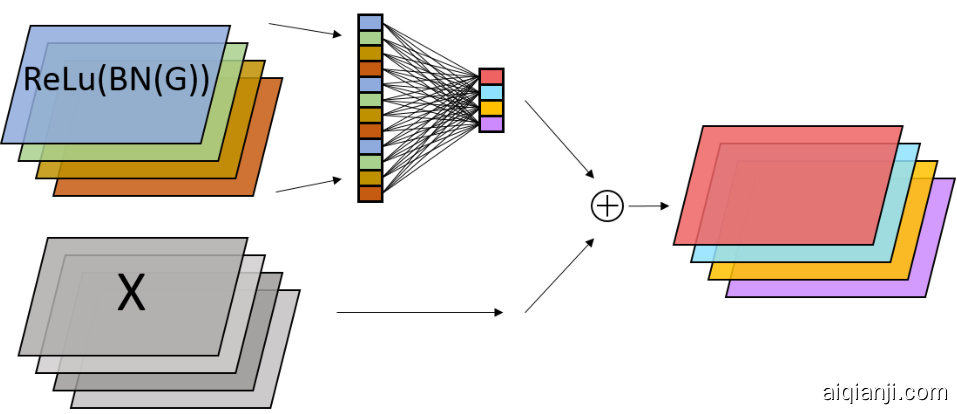
图 1: 示例图片说明
Figure 2: Global pooling bias structure, globally aggregating values of one set of channels to bias another set of channels.
图 2: 全局池化偏置结构,全局聚合一组通道的值以偏置另一组通道。
See Figure 2 for a diagram. This structure follows the first convolution layer of two to three of the residual blocks in KataGo's neural nets, and the frst convolution layer in the policy head. It is also used in the value head with a slight further modification. See Appendix A for details.
见图 2: 为一个示意图。此结构遵循 KataGo 的神经网络中前两个到三个残差块的第一个卷积层,以及策略头的第一个卷积层。它也在价值头中使用,略有进一步修改。详情见附录 A。
In Section 5.2 our experiments show that this greatly improves the later stages of training. As Go contains explicit nonlocal tactics ("ko"), this is not surprising. But global context should help even in domains without explicit nonlocal interactions. For example, in a wide variety of strategy games, strong players, when winning, alter their local move preferences to favor “simple"
在第 5.2 节的实验中,我们显示这大大改善了训练的后期阶段。由于 Go 包含显式的非局部战术 (“ko”),这并不令人惊讶。但是全局上下文即使在没有显式非局部交互的领域也应该有所帮助。例如,在各种战略游戏中,当强者获胜时,他们会改变其局部移动偏好以倾向于“简单”
options, whereas when losing they seek “complication". Global pooling allows convolutional nets to internally condition on such global context.
当获胜时,他们寻求“简化”选项,而当失败时,他们寻求“复杂化”。全局池化允许卷积网络内部根据这种全局上下文进行条件判断。
The general idea of using global context is by no means novel to our work. For example, Hu et al. (2018) have introduced a “Squeeze-and-Excitation” architecture to achieve new results in image classification [8]. Although their implementation is different, the fundamental concept is the same. And though not formally published, Squeeze-Excite-like architectures are now in use in some online AlphaZero-related projects [10, 11], and we look forward to exploring it ourselves in future research.
使用全局上下文的总体思路在我们的工作中绝不是新颖的。例如,Hu 等人 (2018) 引入了 “Squeeze-and-Excitation” 架构,在图像分类方面取得了新成果 [8]。尽管他们的实现方式不同,但基本概念是相同的。虽然尚未正式发布,类似 Squeeze-Excite 的架构已经在一些在线 AlphaZero 相关项目中使用 [10, 11],我们期待在未来的研究中自行探索这一领域。
3.4 Auxiliary Policy Targets
3.4 辅助策略目标
As another general iz able improvement over AlphaZero, we add an auxiliary policy target that predicts the opponent's reply on the following turn to improve regular iz ation. This idea is not entirely new, having been found by Tian and Zhu in Facebook's bot Darkforest to improve supervised move prediction [20], but as far as we know, KataGo is the first to apply it to the AlphaZero process.
作为对 AlphaZero 的另一个通用改进,我们添加了一个辅助策略目标,该目标预测对手在下一轮的回应,以改善正则化。这个想法并不完全新颖,Facebook 的 bot Darkforest 由 Tian 和 Zhu 发现可用于改进监督移动预测 [20],但据我们所知,KataGo 是第一个将其应用于 AlphaZero 过程的。
We simply have the policy head output a new channel predicting this target, adding a term to the loss function:
我们只需让策略头输出一个新的通道来预测这个目标,在损失函数中添加一个项:
$$
-w_{\mathrm{opp}}\sum_{m\in\mathrm{moves}}\pi_{\mathrm{opp}}(m)\log(\hat\pi_{\mathrm{opp}}(m))
$$
where $\pi_{\mathrm{opp}}$ is the policy target that will be recorded for the turn after the current turn, $\hat{\pi}{\mathrm{opp}}$ is the neural net's prediction of $\pi{\mathrm{opp}}$ ,and $w_{\mathrm{opp}}=0.15$ weights this target only a fraction as much as the actual policy, since it is for regular iz ation only and is never actually used for play.
其中,$\pi_{\mathrm{opp}}$ 是当前轮次之后的轮次将要记录的策略目标,$\hat\pi_{\mathrm{opp}}$ 是神经网络对 $\pi_{\mathrm{opp}}$ 的预测,而 $w_{\mathrm{opp}}=0.15$ 表示这个目标的权重仅为实际策略权重的一部分,因为这只是用于正则化,并从未真正用于游戏。
We find in Section 5.2 that this produces a modest but clear benefit. Moreover, this idea could apply to a wide range of reinforcement-learning tasks. Even in single-agent situations, one could predict one's own future actions, or predict the environment (treating the environment as an “agent"). Along with Section 4.1, it shows how enriching the training data with additional targets is valuable when data is limited or expensive. We believe it deserves attention as a simple and nearly costless method to regularize the AlphaZero process or other broader learning algorithms.
我们在第 5.2 节中发现这会产生适度但明显的好处。此外,这个想法可以应用于广泛的强化学习任务。即使在单个 AI 智能体的情况下,也可以预测自己的未来动作,或者预测环境(将环境视为一个“智能体”)。结合第 4.1 节,它展示了在数据有限或昂贵时,通过增加额外目标来丰富训练数据的价值。我们认为这种方法作为一种简单且几乎无成本的方法来规范 AlphaZero 过程或其他更广泛的学习算法,值得重视。
4 Major Domain-Specific Improvements
4 重大领域特定改进
4.1 Auxiliary Ownership and Score Targets
4.1 辅助所有权和得分目标
One of the major improvements in KataGo's training process over AlphaZero comes from adding auxiliary ownership and score prediction targets. Similar targets were earlier explored in work by Wu et al. (2018) [22] in supervised learning, where the authors found improved mean squared error on human game result prediction and mildly improved the strength of their overall bot, CGI.
KataGo 的训练过程相对于 AlphaZero 的一个主要改进是增加了辅助的所有权和得分预测目标。类似的目标 earlier explored in work by Wu et al. (2018) [22] 在监督学习中进行了探索,作者发现对人类比赛结果预测的均方误差有所改善,并轻微提高了他们整体 bot (CGI) 的强度。
To our knowledge, KataGo is the first to publicly apply such ideas to the reinforcement-learninglike context of self-play training in $\mathrm{Go}^{7}$ . While the targets themselves are game-specific, they also highlight a more general heuristic under emphasized in transfer- and multi-task-learning literature.
据我们所知,KataGo 是第一个公开将此类想法应用于 $\mathrm{Go}^{7}$ 自我对弈训练这种强化学习类上下文的。虽然目标本身是特定于游戏的,但它们也突显了在迁移学习和多任务学习文献中被低估的一种更通用的启发式方法。
As observed earlier, in AlphaZero, learning is highly constrained by data and noise on the game outcome prediction. But although the game outcome is noisy and binary, it is a direct function of finer variables: the final score difference and the ownership of each board location8. Decomposing the game result into these finer variables and predicting them as well should improve regular iz ation.
如前所述,在 AlphaZero 中,学习高度受限于数据和游戏结果预测的噪声。但是,尽管游戏结果是嘈杂且二元的,它是更精细变量的直接函数:最终得分差异和每个棋盘位置的所有权8。将游戏结果分解为这些更精细的变量并同时预测它们应该能改善正则化。
Therefore, we add these outputs and three additional terms to the loss function:
因此,我们将这些输出和三个附加项添加到损失函数中:
Ownership loss:
所有权损失:
$$
-w_{o}\sum_{l\in\mathrm{board};p\in\mathrm{players}}o(l,p)\log\left(\hat{o}(l,p)\right)
$$
where $o(l,p)\in{0,0.5,1}$ indicates if $l$ is finally owned by $p$ , or is shared, $\hat{o}$ is the prediction of $o$ , and $w_{o}=1.5/b^{2}$ where $b\in[9,19]$ is the board width.
其中 $o(l,p) \in {0, 0.5, 1}$ 表示位置 $l$ 最终是否被玩家 $p$ 拥有,或共享,$\hat{o}$ 是 $o$ 的预测值,且 $w_{o} = 1.5 / b^{2}$ ,其中 $b \in [9, 19]$ 是棋盘宽度。
Score belief loss ("pdf"):
得分信念损失 ("pdf"):
$$
-w_{\mathrm{spdf}}\sum_{x\in\mathrm{possible~scores}}p_{s}(x)\log(\hat{p}_{s}(x))
$$
where $p_{s}$ is a one-hot encoding of the final score difference, $\hat{p}{s}$ is the prediction of $p{s}$ , and $w_{\mathrm{spdf}}=0.02$
其中,$p_{s}$ 是最终得分差异的 one-hot 编码,$\hat{p}{s}$ 是 $p{s}$ 的预测值,且 $w_{\mathrm{spdf}}=0.02$
Score belief loss ("cdf"):
得分信念损失 ("cdf"):
$$
w_{\mathrm{scdf}}\sum_{x\in\mathrm{possible~scores}}\left(\sum_{y<x}p_{s}(y)-\hat{p}_{s}(y)\right)^{2}
$$
where $w_{\mathrm{scdf}}=0.02$ . While the “pdf" loss rewards guessing the score exactly, this “cdf" loss pushes the overall mass to be near the final score.
其中 $w_\mathrm{scdf} = 0.02$ 。虽然 “pdf” 损失鼓励精确猜测分数,但这种 “cdf” 损失则推动总体分布接近最终分数。
We show in our ablation runs in Section 5.2 that these auxiliary targets noticeably improve the efficiency of learning. This holds even up through the ends of those runs (though shorter, the runs still reach a strength similar to human-professional), well beyond where the neural net must have already developed a sophisticated judgment of the board.
我们在第 5.2 节的消融实验中显示,这些辅助目标显著提高了学习效率。即使在这些实验的后期(尽管时间较短,但实验结果仍然达到了与人类专业水平相近的程度),神经网络显然已经形成了对棋盘复杂的判断力。
It might be surprising that these targets would continue to help beyond the earliest stages. We offer an intuition: consider the task of updating from a game primarily lost due to misjudging a particular region of the board. With only a final binary result, the neural net can only “guess" at what aspect of the board position caused the loss. By contrast, with an ownership target, the neural net receives direct feedback on which area of the board was mis predicted, with large errors and gradients localized to the mis predicted area. The neural net should therefore require fewer samples to perform the correct credit assignment and update correctly.
这些目标在最早阶段之后仍然能提供帮助,这可能令人感到惊讶。我们提供一种直觉理解:考虑从一局主要因为误判了棋盘上某一特定区域而导致失败的游戏进行更新。如果只有最终的二元结果,神经网络只能“猜测”是棋盘上的哪个方面导致了失败。相比之下,通过所有权目标,神经网络可以直接获得关于哪个区域被误预测的反馈,较大的误差和梯度集中在误预测的区域。因此,神经网络应该需要更少的样本来进行正确的信用分配并正确更新。
As with auxiliary policy targets, these results are consistent with work in transfer and multi-task learning showing that adding targets or tasks can improve performance. But the literature is scarcer in theory on when additional targets may help - see Zhang and Yang (2017) [23] for discussion as well as Bingel and Sogaard (2017) [2] for a study in NLP domains. Our results suggest a heuristic: whenever a desired target can be expressed as a sum, conjunction, or disjunction of separate subevents, or would be highly correlated with such subevents, predicting those subevents is likely to help. This is because such a relation should allow for a specific mechanism: that gradients from a mis predicted sub-event will provide sharper, more localized feedback than from the overall event, improving credit assignment.
这些结果与迁移学习和多任务学习中的研究一致,表明添加目标或任务可以提高性能。但是关于何时额外目标可能有所帮助的理论研究较少 - 请参阅 Zhang 和 Yang (2017) [23] 的讨论,以及 Bingel 和 Sogaard (2017) [2] 在 NLP 领域的研究。我们的结果提出了一种启发式方法:每当所需目标可以表示为多个独立子事件的总和、合取或析取,或者与这些子事件高度相关时,预测这些子事件可能会有所帮助。这是因为这种关系应该允许特定机制:来自错误预测子事件的梯度将提供比整体事件更尖锐、更局部化的反馈,从而改善信用分配。

Figure 3: Visualization of ownership predictions by the trained neural net.
图 3: 训练好的神经网络对所有权预测的可视化。
We are likely not the first to discover such a heuristic. And of course, it may not always be applicable. But we feel it is worth highlighting both for practical use and as an avenue for further research, because when applicable, it is a potential path to study and improve the reliability of multi-task-learning approaches for more general problems.
我们可能不是第一个发现这种启发式方法的人。当然,它可能并不总是适用。但我们认为,无论是对于实际应用还是作为进一步研究的方向,都值得强调,因为当适用时,它是研究和改进多任务学习方法可靠性的一个潜在途径,以解决更普遍的问题。
4.2 Game-specific Features
4.2 游戏特定功能
In addition to raw features indicating the stones on the board, the history, and the rules and komi in effect, KataGo includes a few game-specific higher-level features in the input to its neural net, similar to those in earlier work [4, 3, 12]. These features are liberties, komi parity, pass-alive regions, and features indicating ladders (a particular kind of capture tactic). See Appendix A for details.
除了表示棋盘上棋子、历史记录以及当前规则和贴目 (komi) 的原始特征外,KataGo 在输入其神经网络时还包括了一些特定于围棋的高层次特征,类似于早期的工作 [4, 3, 12]。这些特征包括气 (liberties)、贴目奇偶性 (komi parity)、活棋区域 (pass-alive regions) 以及表示打劫 (ladders) 的特征(一种特定的吃子战术)。详情见附录 A。
Additionally, KataGo uses two minor Go-specific optimization s, where after a certain number of consecutive passes, moves in pass-alive territory are prohibited, and where a tiny bias is added to favor passing when passing and continuing play would lead to identical scores. Both optimization s slightly speed up the end of the game.
此外,KataGo 使用了两个次要的围棋特定优化方法,在连续若干次过(pass)之后,禁止在已确定为活棋的区域内落子,并且加入了一个微小的偏置,以在过和继续下棋会导致相同得分的情况下更倾向于过。这两种优化方法略微加快了游戏结束的速度。
To measure the effect of these game-specific features and optimization s, we include in Section 5.2 an ablation run that disables both ending optimization s and all input features other than the locations of stones, previous move history, and game rules. We find they contribute noticeably to the learning speed, but account for only a small fraction of the total improvement in KataGo.
为了测量这些特定于游戏的特征和优化的效果,我们在第 5.2 节中包含了一个消融实验,该实验禁用了结束优化以及除石头位置、先前移动历史和游戏规则之外的所有输入特征。我们发现它们对学习速度有明显贡献,但仅占KataGo总改进的一小部分。
5 Results
5.1 Testing Versus ELF and Leela Zero
5.1 对战 ELF 和 Leela Zero
We tested KataGo against ELF and Leela Zero 0.17 using their publicly-available source code and trained networks.
我们使用公开可用的源代码和训练网络对 KataGo 进行了测试,测试对象为 ELF 和 Leela Zero 0.17。
We sampled roughly every fifth Leela Zero neural net over its training history from “LZ30" through "LZ225", the last several networks well exceeding even ELF's strength. Between every pair of Leela Zero nets fewer than 35 versions apart, we played about 45 games to establish approximate relative strengths of the Leela Zero nets as a benchmark.
我们大约每隔五个 Leela Zero 神经网络在其训练历史中进行采样,从 “LZ30” 到 “LZ225”,最后几个网络的强度甚至超过了 ELF。对于每对间隔少于 35 个版本的 Leela Zero 网络,我们进行了大约 45 场对局,以建立 Leela Zero 网络之间的相对强度作为基准。
We also sampled KataGo over its training history, for each version playing batches of games versus random Leela Zero nets with frequency proportional to the predicted variance $p(1-p)$ of the game result. The winning chance $p$ was continuously estimated from the global Bayesian maximumlikelihood Elo based on all game results so far9. This ensured that games would be varied yet informative. We also ran ELF's final "V2" neural network using Leela Zero's engine $_{10}$ ,withELF playing against both Leela Zero and KataGo using the same opponent sampling.
我们还根据 KataGo 的训练历史进行了采样,每个版本与随机的 Leela Zero 网络对战一批游戏,频率与预测的游戏结果方差 $p(1-p)$ 成正比。胜率 $p$ 通过迄今为止所有比赛结果的全局贝叶斯最大似然 Elo 进行了连续估计 [9]。这确保了游戏既多样化又有信息量。我们还使用 Leela Zero 的引擎运行了 ELF 的最终“V2”神经网络 [10],ELF 与 Leela Zero 和 KataGo 对战时使用相同的对手采样方法。
Games used a 19x19 board with a fixed 7.5 komi under Tromp-Taylor rules, with a fixed 1600 visits, resignation below 2% winrate, and multithreading disabled. To encourage opening variety, both bots randomized with a temperature of 0.2 in the first 20 turns. Both also used a “lowerconfidence-bound" move selection method to improve match strength [15]. Final Elo ratings were based on the final set of about 21000 games.
游戏使用了 19x19 的棋盘,采用 Tromp-Taylor 规则,固定贴目 7.5,每局固定 1600 次访问,胜率低于 2% 时认输,并且禁用多线程。为了鼓励开局多样性,两个机器人在前 20 步中以温度 0.2 进行随机化。两者还使用了“lowerconfidence-bound”移动选择方法来提高比赛强度 [15]。最终的 Elo 评级基于大约 21000 局游戏的最终结果。
To compare the efficiency of training, we computed a crude indicative metric of total self-play com putation by modeling a neural net with $b$ blocks and $c$ channels as having cost $\sim b c^{2}$ per queryll. For KataGo we just counted self-play queries for each size and multiplied. For ELF, we approximated queries by sampling the average game length from its public training data and multiplied by ELF's 1600 playouts per move, discounting by 20% to roughly acount for transposition caching. For Leela Zero we estimated it similarly, also interpolating costs where data was missingl2. Leela. Zero also generated data using ELF's prototype networks, but we did not attempt to estimate this cost13.
为了比较训练效率,我们计算了一个粗略的指示性指标,即通过建模一个具有 $b$ 个块和 $c$ 个通道的神经网络,其每次查询的成本为 $\sim b c^{2}$,来估算总的自我对弈计算量。对于 KataGo,我们只是统计了每个规模的自我对弈查询并相乘。对于 ELF,我们通过采样其公开训练数据中的平均游戏长度来近似查询次数,并乘以 ELF 每步的 1600 次模拟,再减少 20% 以大致考虑变位缓存的影响。对于 Leela Zero,我们进行了类似的估算,在数据缺失的地方也进行了成本插值。Leela Zero 还使用了 ELF 的原型网络生成了数据,但我们没有尝试估算这部分成本。
KataGo compares highly favorably with both ELF and Leela Zero. Shown in Figure 4 is a plot of Elo ratings versus estimated compute for all three. KataGo outperforms ELF in learning efficiency under this metric by about a factor of 50. Leela Zero appears to outperform ELF as well, but the Elo ratings would be expected to unfairly favor Leela since its final network size is 40 blocks, double
KataGo 与 ELF 和 Leela Zero 相比具有显著优势。图 4 显示了这三者的 Elo 评分与估计计算量的对比图。在此指标下,KataGo 的学习效率比 ELF 高出约 50 倍。Leela Zero 似乎也优于 ELF,但 Elo 评分可能不公平地偏向 Leela,因为其最终网络大小为 40 个块,是 ELF 的两倍。
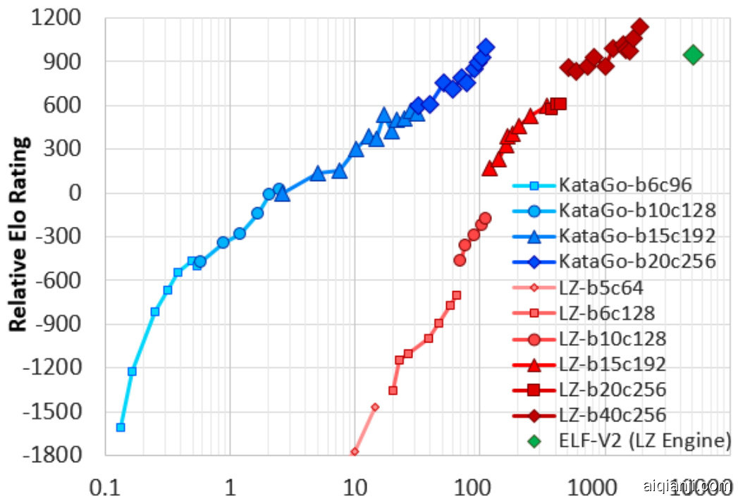
Figure 4: 1600-visit Elo progression of KataGo (blue, leftmost) vs. Leela Zero (red, center) and ELF (green diamond). X-axis: self-play cost in billions of equivalent 20 block x 256 channel queries. Note the log-scale. Leela Zero's costs are highly approximate.
图 4: KataGo (蓝色,最左侧) 在 1600 次访问中的 Elo 进展与 Leela Zero (红色,中间) 和 ELF (绿色菱形) 的对比。X 轴:以数十亿个等效于 20 层 x 256 通道查询的自我对弈成本表示。注意对数刻度。Leela Zero 的成本是高度估算的。
| 对战设置 | 对 ELF 的胜场数 | Elo 分差 |
|---|---|---|
| 1600 次模拟,mV 1 不批处理 | 239 400 | 69 ± 36 |
| 9.0 秒 mv,ELF 批处理大小 16 | 246 400 | 81 ± 36 |
| 7.5 秒 mv,ELF 批处理大小 32 | 254 1/4 400 | 96 ± 37 |
that of ELF, and the ratings are based on equal search nodes rather than GPU cost. Additionally, Leela Zero's training occurred over multiple years rather than ELF's two weeks, reducing latency and parallel iz ation overhead. Yet KataGo still outperforms Leela Zero by a factor of 10 despite the same network size as ELF and a similarly short training time. Early on, the improvement factor appears larger, but partly this is because the first 10%-15% of Leela Zero's run contained some bugs that slowed learning.
其与 ELF 相同,评级是基于相同的搜索节点而不是 GPU 成本。此外,Leela Zero 的训练历时多年,而 ELF 仅用两周,减少了延迟和平行化开销。尽管 KataGo 与 ELF 拥有相同的网络规模,并且训练时间同样短暂,但 KataGo 的性能仍比 Leela Zero 高出 10 倍。在早期,改进因子看起来更大,但这部分是因为 Leela Zero 的前 10%-15% 的运行中存在一些 bug,减慢了学习速度。
We also ran three 400-game matches on a single V100 GPU against ELF using ELF's native engine. In the frst, both sides used 1600 playouts/move with no batching. In the second, KataGo used 9s/move (16 threads, max batch size 16) and ELF used 16,000 playouts/move (batch size 16), which ELF performs in 9 seconds. In the third, we doubled ELF's batch size, improving its nominal speed to 7.5s/move, and lowered KataGo to 7.5s/move. As summarized in Table 1, in all three matches KataGo defeated ELF, confrming its strength level at both low and high playouts and at both fixed search and fixed wall clock time settings.
我们还在单个 V100 GPU 上与使用 ELF 的原生引擎进行了三场 400 局的比赛。在第一场比赛中,双方每步使用 1600 次模拟且不进行批处理。在第二场比赛中,KataGo 使用 9 秒/步(16 线程,最大批处理大小为 16),而 ELF 使用 16,000 次模拟/步(批处理大小为 16),这在 9 秒内完成。在第三场比赛中,我们将 ELF 的批处理大小加倍,将其名义速度提高到 7.5 秒/步,并将 KataGo 降低到 7.5 秒/步。如表 1 所示,在所有三场比赛中,KataGo 均击败了 ELF,确认了其在低和高模拟次数以及固定搜索时间和固定墙钟时间设置下的强度水平。
5.2 Ablation Runs
5.2 消融实验
To study the impact of the techniques presented in this paper, we ran shorter training runs with various components removed. These ablation runs went for about 2 days each, with identical parameters except for the following differences:
为了研究本文提出的技术的影响,我们进行了较短的训练运行,并移除了不同的组件。这些消融实验每次大约进行了2天,参数相同,但有以下差异:
We sampled neural nets from these runs together with KataGo's main run, and evaluated them the same way as when testing against Leela Zero and ELF: playing $19\mathrm{x19}$ games between random versions based on the predicted variance $p(1-p)$ of the result. Final Elos are based on the final set of about 147,000 games (note that these Elos are not directly comparable to those in Section 5.1).
我们从这些运行中以及KataGo的主要运行中采样了神经网络,并以与测试Leela Zero和ELF相同的方式评估它们:在基于预测结果方差 $p(1-p)$ 的随机版本之间进行 $19\times19$ 对局。最终的Elo分数是基于最后大约147,000局游戏的结果(注意,这些Elo分数不能直接与第5.1节中的进行比较)。
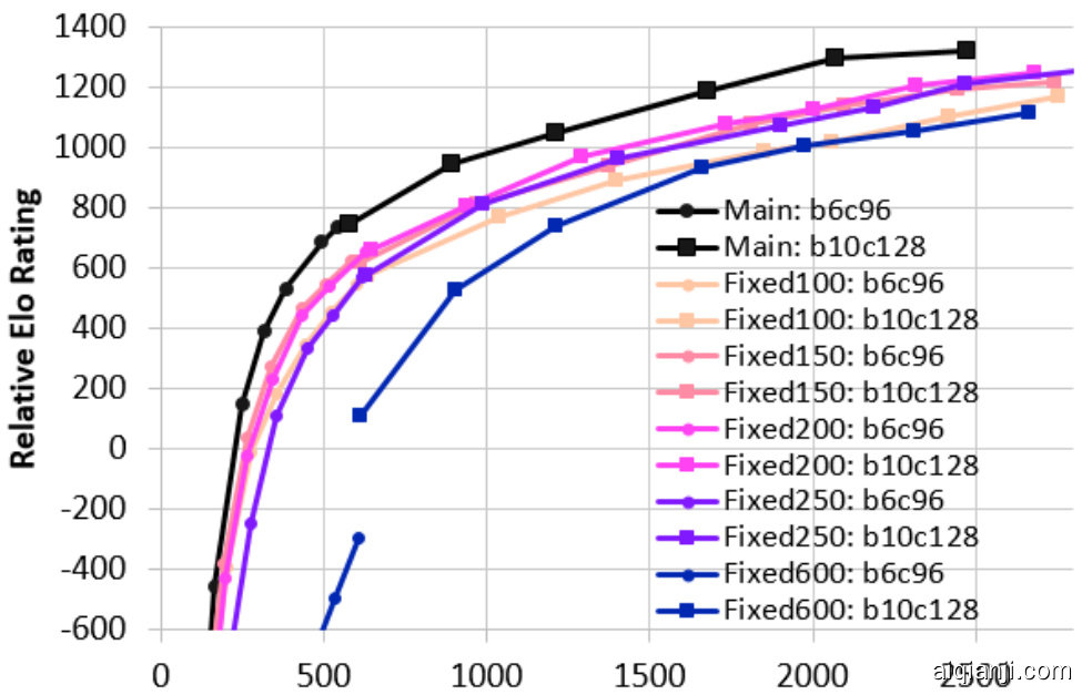
Figure 5: KataGo's main run versus Fixed runs. X-axis is the cumulative self-play cost in millions of equivalent 20 block $\mathrm{x256~}$ channel queries.
图 5: KataGo 的主要运行与固定运行的对比。X 轴是累积的自我对弈成本,单位为相当于 20 层 × 256 通道查询的百万次。
As shown in Figure 5, playout cap random iz ation clearly outperforms a wide variety of possible fixed values of playouts. This is precisely what one would expect if the technique relieves the tension between the value and policy targets present for any fixed number of playouts. Interestingly, the
如图 5 所示,落子上限随机化 (playout cap randomization) 明显优于各种可能的固定落子数。这正是人们期望的结果,如果该技术能够缓解任何固定落子数下价值目标和策略目标之间的矛盾。有趣的是,
Figure 5: 落子上限随机化与固定落子数的性能对比
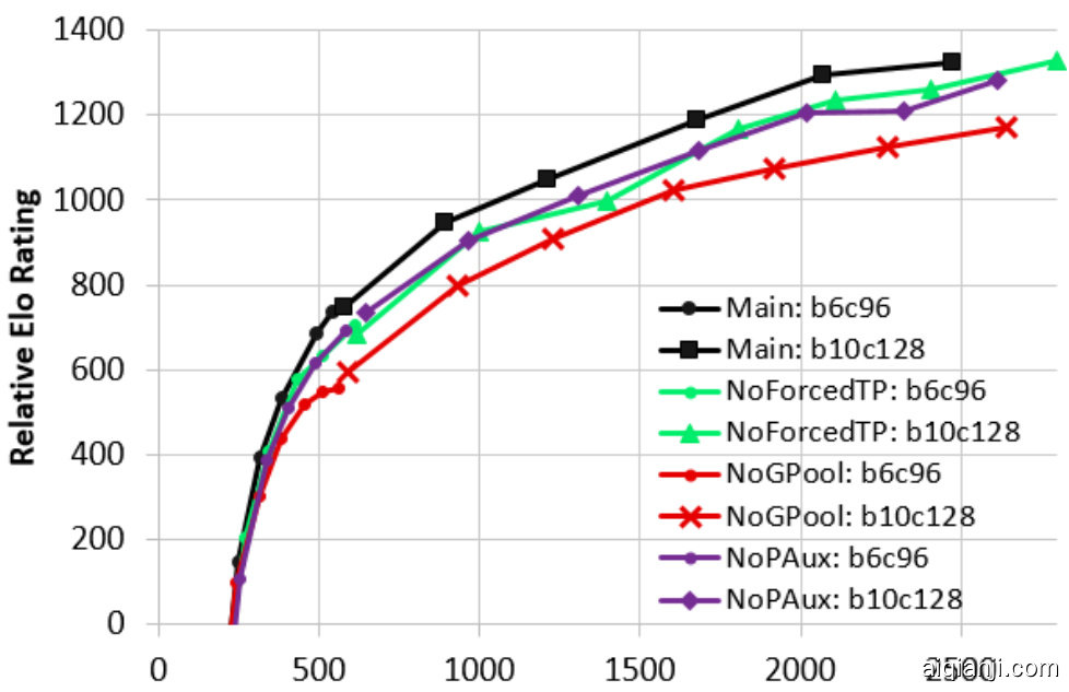
Figure 6: KataGo's main run versus NoGPool, NoForcedTP, NoPAux. X-axis is the cumulative self-play cost in millions of equivalent 20 block $\mathrm{x256~}$ channel queries.
图 6: KataGo 的主要运行与 NoGPool, NoForcedTP, NoPAux 的对比。X 轴是累积的自我对弈成本,以百万个等效于 20 层 × 256 通道查询为单位。
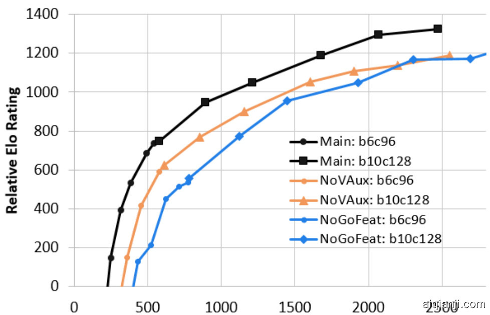
Figure 7: KataGo's main run versus NoVAux, NoGoFeat. X-axis is the cumulative self-play cost in millions of equivalent 20 block $\mathrm{x256~}$ channel queries.
图 7: KataGo 的主要运行与 NoVAux、NoGoFeat 的对比。X 轴是累计自我对弈成本,单位为相当于 20 层 × 256 通道查询的百万次。
600-playout run showed a large jump in strength when increasing neural net size. We suspect this is due to poor convergence from early over fitting not entirely mitigated by doubling the training window.
600 次模拟运行显示,当增加神经网络规模时,性能有了显著提升。我们怀疑这是由于早期过拟合导致的收敛不良,即使将训练窗口翻倍也未能完全缓解这个问题。
As shown in Figure 6, global pooling noticeably improved learning efficiency, and forced playouts with policy target pruning and auxiliary policy targets also provided smaller but clear gains. Inte rest ingly, all three showed little effect early on compared to later in the run. We suspect their relative value continues to increase beyond the two-day mark at which we stopped the ablation runs. These plots suggest that the total value of these general enhancements to self-play learning, along with playout cap random iz ation, is large.
如图 6 所示,全局池化显著提高了学习效率,带有策略目标剪枝和辅助策略目标的强制推演也提供了较小但明显的效果改进。有趣的是,这三种方法在运行初期相比后期表现出的效果较小。我们怀疑它们的相对价值在我们停止消融实验的两天标记之后会继续增加。这些图表表明,这些对自我对弈学习的通用增强方法的总价值,以及推演上限随机化,是巨大的。
As shown in Figure 7, removing auxiliary ownership and score targets resulted in a noticeable drop in learning efficiency. These results confrm the value of these auxiliary targets and the value, at least in Go, of regular iz ation by predicting sub components of targets. Also, we observe a drop in efficiency from removing Go-specific input features and optimization s, demonstrating that there is still significant value in such domain-specific methods, but also accounting for only a part of the total speedup achieved by KataGo.
如图 7 所示,移除辅助所有权和得分目标导致学习效率显著下降。这些结果确认了这些辅助目标的价值,以及至少在 Go 中,通过预测目标的子组件进行正则化的价值。此外,我们观察到移除 Go 特定的输入特征和优化方法后效率下降,这表明此类领域特定方法仍然具有重要价值,但也只解释了 KataGo 实现的总加速的一部分。
See Table 2 for a summary. The product of the acceleration factors shown is approximately 9.1x. We suspect this is an underestimate of the true speedup since several techniques continued to increase in effectiveness as their runs progressed and the ablation runs were shorter than our full run. Some remaining differences with ELF and/or AlphaZero are likely due to infrastructure and implementation. Unfortunately, it was beyond our resources to replicate ELF and/or AlphaZero's infrastructure of thousands of GPUs/TPUs for a precise comparison, or to run more extensive ablation runs each for as long as would be ideal.
见表 2: 总结。所示加速因子的乘积约为 9.1倍。我们怀疑这是对实际加速比的低估,因为一些技术在其运行过程中继续提高效果,而消融实验的运行时间比完整运行时间短。与 ELF 和/或 AlphaZero 的一些剩余差异可能归因于基础设施和实现的不同。遗憾的是,我们的资源无法复制 ELF 和/或 AlphaZero 的数千个 GPU/TPU 基础设施以进行精确比较,也无法运行更长时间的理想消融实验。
| 移除的组件 | Elo | 因子 |
|---|---|---|
| (主运行,基准) Playout Cap Randomization F.P. 和策略目标修剪 全局池化 辅助策略目标 辅助 x 所有者和得分目标 游戏特定特征 | 1329 1242 1276 1153 1255 1139 1 Opts 1168 | 1.00x 1.37x 1.25x 1.60x 1.30x 1.65x 1.55x |
Table 2: For each technique, the Elo of the ablation run omitting it as of reaching 2.5G equivalent 20b x 256c self-play queries ( $\approx2$ days), and the factor increase in training time to reach that Elo. Factors are app roc i mate and are based on shorter runs.
表 2: 对于每种技术,在达到相当于 2.5G 的 20b x 256c 自我对局查询 (≈2 天) 时,省略该技术的消融运行的 Elo,以及达到该 Elo 所需的训练时间增加倍数。倍数是近似的,基于较短的运行结果。
6 Conclusions And Future Work
6 结论与未来工作
Still beginning only from random play with no external data, our bot KataGo achieves a level competitive with some of the top AlphaZero replications, but with an enormously greater efficiency than all such earlier work. In this paper, we presented a variety of techniques we used to improve self-play learning, many of which could be readily applied to other games or to problems in reinforcement learning more generally. Furthermore, our domain-specific improvements demonstrate a remaining gap between basic AlphaZero-like training and what could be possible, while also suggesting principles and possible avenues for improvement in general methods. We hope our work lays a foundation for further improvements in the data efficiency of reinforcement learning.
仍然仅从随机游戏开始且没有外部数据,我们的机器人 KataGo 达到了与一些顶级 AlphaZero 复制品相当的水平,但效率远高于所有先前的工作。在本文中,我们介绍了用于改进自我对弈学习的各种技术,其中许多可以很容易地应用于其他游戏或更广泛的强化学习问题。此外,我们的领域特定改进表明了基本的 AlphaZero 类训练方法与可能实现的目标之间仍存在差距,同时也提出了改进通用方法的原则和可能途径。我们希望我们的工作为提高强化学习的数据效率奠定了基础。
References
参考文献
Appendix A Neural Net Inputs and Architecture
The following is a detailed breakdown of KataGo's neural net inputs and architecture. The neural net has two input tensors, which feed into a trunk of residual blocks. Attached to the end of the trunk are a policy head and a value head, each with several outputs and sub components.
以下是 KataGo 的神经网络输入和架构的详细分解。该神经网络有两个输入张量,它们馈入一个残差块组成的主干。在主干的末端连接着一个策略头 (policy head) 和一个价值头 (value head),每个头都有多个输出和子组件。
A.1 Inputs
A.1 输入
The input to the neural net consists of two tensors, a $b\times b\times18$ tensor of 18 binary features for each board location where where $b\in[b_{\operatorname*{min}},b_{\operatorname*{max}}]=[9,19]$ is the width of the board, and a vector with 10 real values indicating overall properties of the game state. These features are summarized in Tables 3 and 4
输入到神经网络的包括两个张量,一个是每个棋盘位置包含 18 个二进制特征的 $b\times b\times18$ 张量,其中 $b\in[b_{\operatorname*{min}},b_{\operatorname*{max}}]=[9,19]$ 是棋盘的宽度,另一个是包含 10 个实数值的向量,表示游戏状态的整体属性。这些特征在表 3 和表 4 中进行了总结。
| # 通道 | 特征 |
|---|---|
| 1 | 位置在棋盘上 |
| 2 | 位置有 {己方,对方} 的棋子 |
| 3 | 位置有带有 {1,2,3} 气的棋子 |
| 1 | 移动到这里由于 Ko/超级 Ko 而非法 |
| 5 | 最后 5 步移动的位置,独热编码 |
| 3 | 可以形成阶梯的棋子在 {0,1,2} 步之前 |
| 1 | 移动到这里可以将对方困在阶梯中 |
| 2 | 对于 {自己,对方} 的无眼活区域 |
Table 3: Binary spatial-varying input features to the neural net. A “ladder” occurs when stones are forcibly capturable via consecutive inescapable atari (i.e. repeated capture threat).
表 3: 输入神经网络的二进制空间变化特征。当石头通过连续不可避免的打吃 (即重复的捕获威胁) 被强制捕获时,称为“梯形”。
Table 4: Overall game state input features to the neural net.
表 4: 输入神经网络的整体游戏状态特征。
| # Channels | 特征 |
|---|---|
| 5 | 前 5 步中哪一步是 pass? |
| 1 | 贴目 15.0 (当前玩家视角) |
| 2 | 禁入点规则 (简单, 位置, 情境) |
| 1 | 是否允许自杀? |
| 1 | 贴目 + 棋盘大小奇偶性 |
A.2 Global Pooling
A.2 全局池化
Certain layers in the neural net are global pooling layers. Given a set of $c$ channels, a global pooling layer computes:
神经网络中的某些层是全局池化层。给定一组 $c$ 个通道,一个全局池化层计算:
where $b_{\mathrm{avg}}=0.5(b_{\mathrm{min}}+b_{\mathrm{max}})=0.5(9+19)$ . This produces a total of $3c$ output values. The multiplication in (2) allows training weights that work across multiple board sizes, and the subtraction of $b_{\mathrm{avg}}$ and scaling by $1/10$ improve orthogonality and ensure values remain near unit scale. In the value head, (3) is replaced with the mean of each channel multiplied by $\textstyle{\frac{1}{100}}((b-b_{\mathrm{avg}})^{2}-\sigma^{2})$ where $\begin{array}{r}{\sigma^{2}=\frac{1}{11}\sum_{b^{\prime}=9}^{19}(b^{\prime}-b_{\mathrm{avg}})^{2}}\end{array}$ . This is since the value head computes values like score difference that need to scale quadratically with board width. As before, subtracting $\sigma^{2}$ and scaling improves orthogonality and normality.
其中 $b_{\mathrm{avg}}=0.5(b_{\mathrm{min}}+b_{\mathrm{max}})=0.5(9+19)$ 。这产生了总共 $3c$ 个输出值。公式 (2) 中的乘法允许训练适用于多个棋盘大小的权重,减去 $b_{\mathrm{avg}}$ 并按 $1/10$ 缩放可以提高正交性并确保值保持在单位尺度附近。在价值头中,(3) 被替换为每个通道的平均值乘以 $\textstyle{\frac{1}{100}}((b-b_{\mathrm{avg}})^{2}-\sigma^{2})$ ,其中 $\begin{array}{r}{\sigma^{2}=\frac{1}{11}\sum_{b^{\prime}=9}^{19}(b^{\prime}-b_{\mathrm{avg}})^{2}}\end{array}$ 。这是因为价值头计算诸如分数差异之类的值,这些值需要与棋盘宽度成二次方关系缩放。同样,减去 $\sigma^{2}$ 和缩放可以改善正交性和正态性。
Using such layers, a global pooling bias structure takes input tensors $X$ (shape $b\times b\times c_{X}$ ) and $G$ (shape $b\times b\times c_{G}$ ) and consists of:
使用此类层,全局池化偏置结构接收输入张量 $X$ (形状为 $b\times b\times c_X$ ) 和 $G$ (形状为 $b\times b\times c_G$ ),并由以下部分组成:
A.3 Trunk
A.3 主干
The trunk consists of:
主干包含:
● The remaining two or three blocks, spaced at regular intervals in the trunk, use global pooling, consisting of the following in order:
● 剩余的两到三个块,以固定间隔分布在主干中,使用全局池化,按顺序包括以下内容:
· At the end of the trunk, a batch-normalization layer and one more ReLU activation function.
在主干的末尾,一个批归一化层和一个 ReLU 激活函数。
A.4 Policy Head
A.4 策略头 (Policy Head)
The policy head consists of:
策略头包括:
A.5 Value Head
A.5 价值头 (Value Head)
The value head consists of:
值头由以下部分组成:
· A 1x1 convolution outputting $c_{\mathrm{head}}$ channels ("V").
1x1 卷积输出 $c_{\mathrm{head}}$ 通道 (“V”)。
· A global pooling layer of $V$ outputting $3c_{\mathrm{head}}$ values (*"Vpooled").
全局池化层对 $V$ 输出 $3c_{\mathrm{head}}$ 个值 (*"Vpooled")。
- A game-outcome subhead consisting of: - A fully-connected layer from $V_{\mathrm{pooled}}$ including bias terms outputting $c_{\mathrm{val}}$ values. - A ReLU activation function. - A fully-connected layer from $V_{\mathrm{pooled}}$ including bias terms outputting 9 values.
- The first 3 values are a distribution in logits whose softmax $\hat{z}$ predicts among the three possible game outcomes win, loss, and no result (the latter being possible under non-superko rulesets in case of long-cycles).
- The fourth value is multiplied by 20 to produce a prediction $\hat{\mu}_{s}$ of the final score difference of the game in points $^{14}$
游戏结果子标题包括:
- 从 $V_{\mathrm{pooled}}$ 输出 $c_{\mathrm{val}}$ 值的全连接层,包含偏置项。
- ReLU 激活函数。
- 从 $V_{\mathrm{pooled}}$ 输出 9 个值的全连接层,包含偏置项。
- 前 3 个值是 logits 分布,其 softmax $\hat{z}$ 预测三种可能的游戏结果:胜、负和无结果(后者在非超级劫规则集下可能出现长循环时)。
- 第 4 个值乘以 20 以生成对最终得分差异的预测 $\hat{\mu}_{s}$,单位为点数 $^{14}$。
- The fifth value has a softplus activation applied and is then multiplied by 20 to produce an estimate $\sigma_{s}$ of the standard deviation of the predicted final score difference in points. The sixth through ninth values have a softplus activation applied are predictions $\hat{\mathbf{r}}\hat{\mathbf{v}}_{i}$ of the expected variance in the MCTS root value for different numbers of playouts.
- All predictions are from the perspective of the current player.
- 第五个值应用了 softplus 激活函数,然后乘以 20,以生成预测最终得分差异标准差的估计值$\sigma_{s}$。第六个到第九个值应用了 softplus 激活函数,是对不同模拟次数的 MCTS 根值预期方差的预测 $\hat{\mathbf{r}}\hat{\mathbf{v}}_{i}$。
- 所有预测均从当前玩家的角度进行。
● An ownership subhead consisting of:
● 一个所有权副标题,包含以下内容:
· A final-score-distribution subhead consisting of:
最终得分分布子标题由以下内容组成:
- A scaling component:
- 一个缩放组件:
* A fully-connected layer from $V_{p o o l e d}$ including bias terms outputting $c_{\mathrm{val}}$ values. * A ReLU activation function. * A fully-connected layer including bias terms outputting 1 value $(\stackrel{\leftarrow}{\gamma})$
- 从 $V_{p o o l e d}$ 输出 $c_{\mathrm{val}}$ 值的全连接层 (包括偏置项)。
- ReLU 激活函数。
- 输出 1 个值 $(\stackrel{\leftarrow}{\gamma})$ 的全连接层 (包括偏置项)。
- For each possible final score value $s$
- 对于每个可能的最终得分值 $s$
$$
s\in{-S+0.5,-S+1.5,\ldots,S-1.5,S-0.5}
$$
where $S$ is a an upper bound for the plausible final score difference of any game $^{16}$ ,in parallel:
其中 $S$ 是任何比赛合理最终得分差异的上限 $^{16}$ ,并行地:
$^*$ The $3c_{\mathrm{head}}$ values from $V_{p o o l e d}$ are concatenated with two additional values:
$^*$ 来自 $V_{p o o l e d}$ 的 $3c_{\mathrm{head}}$ 值与两个附加值连接:
请注意,这里包含了一些特殊的数学符号和公式,按照规则1,这些特殊字符和公式保持原样未进行翻译。
$$
(0.05*s,\mathrm{Parity}(s)-0.5)
$$
0.05 is an arbitrary reasonable scaling factor so that these values vary closer to unit scale. Parity(s) is the binary indicator of whether a score value is normally possible or not due to parity of the board size and komi17.
0.05 是一个任意的合理缩放因子,使得这些值更接近单位尺度。Parity(s) 是分数值是否由于棋盘大小和贴目17 (komi17) 的奇偶性而正常可能的二进制指示器。
- The resulting $2S$ values multiplied by softplus( $\gamma$ )are a distribution in logits whose softmax $\hat{p}_{s}$ predicts the final score difference of the game in points. All predictions are from the perspective of the current player.
- 所得的 $2S$ 值乘以 softplus( $\gamma$ ) 是一个 logits 分布,其 softmax $\hat{p}_{s}$ 预测比赛的最终得分差异(以分计)。所有预测均从当前玩家的角度出发。
A.6 Neural Net Parameters
A.6 神经网络参数
Four different neural net sizes were used in our experiments. Table 5 summarizes the constants for each size. Additionally, the four different sizes used, respectively, 2, 2, 2, and 3 global pooling residual blocks in place of ordinary residual blocks, at regularly spaced intervals.
在我们的实验中使用了四种不同大小的神经网络。表 5: 总结了每个大小的常量。此外,分别使用了 2、2、2 和 3 个全局池化残差块代替普通残差块,间隔均匀分布。
Table 5: Architectural constants for various neural net sizes.
表 5: 不同神经网络大小的架构常数。
| Size | b6×c96 | b10xc128 | b15xc192 | b20xc256 |
|---|---|---|---|---|
| n | 6 | 10 | 15 | 20 |
| C | 96 | 128 | 192 | 256 |
| Cpool | 32 | 32 | 64 | 64 |
| Chead | 32 | 32 | 32 | 48 |
| Cval | 48 | 64 | 80 | 96 |
Appendix B Loss Function
附录 B 损失函数
The loss function used for neural net training in KataGo is the sum of:
KataGo 中用于神经网络训练的损失函数是以下各项的总和:
Game outcome value loss:
游戏结果值损失:
$$
c_{\mathrm{value}}\sum_{r\in{\mathrm{win,loss}}}z(r)\log(\hat{z}(r))
$$
where $\mathcal{Z}$ is a one-hot encoding of whether the game was won or lost by the current player, $\hat{z}$ is the neural net's prediction of $z$ ,and $c_{\mathrm{value}}=1.5$
其中 $\mathcal{Z}$ 是当前玩家胜负情况的 one-hot 编码,$\hat{z}$ 是神经网络对 $z$ 的预测,$c_{\mathrm{value}}=1.5$
· Policy loss:
· 策略损失:
政策损失 (Policy loss):
$$
-\sum_{m\in\mathrm{moves}}\pi(m)\log(\hat{\pi}(m))
$$
where $\pi$ is the target policy distribution and $\hat\pi$ is the prediction of $\pi$
其中 $\pi$ 是目标策略分布,$\hat\pi$ 是 $\pi$ 的预测
● Opponent policy loss:
● 对手策略损失:
$$
-w_{\mathrm{opp}}\sum_{m\in\mathrm{moves}}\pi_{\mathrm{opp}}(m)\log(\hat\pi_{\mathrm{opp}}(m))
$$
where $\pi_{\mathrm{opp}}$ is the target opponent policy distribution, $\hat\pi_{\mathrm{opp}}$ is the prediction of $\pi_{\mathrm{opp}}$ , and $w_{\mathrm{opp}}=0.15$
其中,$\pi_{\mathrm{opp}}$ 是目标对手策略分布,$\hat\pi_{\mathrm{opp}}$ 是 $\pi_{\mathrm{opp}}$ 的预测,$w_{\mathrm{opp}} = 0.15$。
Ownership loss:
所有权损失:
$$
-w_{o}\sum_{l\in\mathrm{board};p\in\mathrm{players}}o(l,p)\log\left(\hat{o}(l,p)\right)
$$
where $o(l,p)\in{0,0.5,1}$ indicates if $l$ is finally owned by $p$ , or is shared, $\hat{o}$ is the prediction of $o$ , and $w_{o}=1.5/b^{2}$ where $b\in[9,19]$ is the board width.
其中 $o(l,p)\in{0,0.5,1}$ 表示位置 $l$ 最终是否被玩家 $p$ 所拥有,或共享,$\hat{o}$ 是 $o$ 的预测值,且 $w_{o}=1.5/b^{2}$ ,其中 $b\in[9,19]$ 是棋盘宽度。
Score belief loss (“pdf"):
得分信念损失 (“pdf”)
$$
-w_{\mathrm{spdf}}\sum_{x\in\mathrm{possible~scores}}p_{s}(x)\log(\hat{p}_{s}(x))
$$
where $p_{s}$ is a one-hot encoding of the final score difference, $\hat{p}{s}$ is the prediction of $p{s}$ ,and $w_{\mathrm{spdf}}=0.02$
其中,$p_{s}$ 是最终得分差异的 one-hot 编码,$\hat{p}{s}$ 是 $p{s}$ 的预测值,且 $w_{\mathrm{spdf}}=0.02$
Score belief loss ("cdf"):
得分信念损失 ("cdf"):
$$
w_{\mathrm{scdf}}\sum_{x\in\mathrm{possible~scores}}\left(\sum_{y<x}p_{s}(y)-\hat{p}_{s}(y)\right)^{2}
$$
where $w_{\mathrm{scdf}}=0.02$
其中 $w_{\mathrm{scdf}}=0.02$
· Score belief mean self-prediction:
得分信念均值自我预测:
$$
-w_{sbreg} Huber(\hat{\mu}_{s}-\mu_s,,\delta=10.0)
$$
where $w_{\mathrm{sbreg}}=0.004$ and
其中 $w_{\mathrm{sbreg}}=0.004$ 和
请注意,您提供的内容似乎是一段公式或参数设置的一部分,没有更多的上下文信息。如果您有更多需要翻译的内容或者具体的句子,请提供完整的信息以便进行准确翻译。
$$
\mu_{s}=\sum_{x}x\hat{p}_{s}(x)
$$
and $\operatorname{Huber}(x,\delta)$ is the Huber loss function equal to the squared error loss $f(x),=,1/2x^{2}$ except that for $|x|>\delta$ ,instead $\begin{array}{r}{\mathrm{Huber}(x,\delta)=f(\delta)+(|x|-\delta)\frac{d f}{d x}(\delta)}\end{array}$ . This avoids some cases of divergence in training due to large errors just after initialization, but otherwise is exactly identical to a plain squared error beyond the earliest steps of training.
和 $\operatorname{Huber}(x,\delta)$ 是 Huber 损失函数,等于平方误差损失 $f(x),=,1/2x^{2}$,除了当 $|x|>\delta$ 时,
$\begin{array}{r}{\mathrm{Huber}(x,\delta)=f(\delta)+(|x|-\delta)\frac{d f}{d x}(\delta)}\end{array}$。
这避免了由于初始化后出现较大误差而导致训练中的一些发散情况,但在训练的最初几步之外,它与普通的平方误差完全相同。
Note that neural net is predicting itself - i.e. this is a regular iz ation term for an otherwise unanchored output $\hat{\mu}_{s}$ to roughly equal to the mean score implied by the neural net's full score belief distribution. The neural net easily learns to make this output highly consistent with its own score belief18.
请注意,神经网络是在预测自身——即这是一个正则化项,用于使原本未固定的输出 $\hat{\mu}_{s}$ 大致等于神经网络的完整评分信念分布所隐含的平均分数。神经网络很容易学习使这个输出与其自身的评分信念高度一致[18]。
· Score belief standard deviation self-prediction:
得分信念标准差自预测:
$$
- w_{sbreg} Huber(\hat{\sigma}_s - \sigma_s,,\delta = 10.0)
$$
where
哪里
根据提供的规则和策略,以上仅是单词 "where" 的直接翻译。但是,如果 "where" 是在句子或段落中的一部分,请提供完整的上下文以便进行准确的翻译。
$$
\sigma_{s}=\left(\sum_{x}(x-\mu)^{2}\hat{p}_{s}(x)\right)^{1/2}
$$
Similarly, the neural net is predicting itself - i.e. this is a regular iz ation term for an otherwise unanchored output $\hat{\sigma}_{s}$ to roughly equal to the standard deviation of the neural net's full score belief distribution. The neural net easily learns to make this output highly consistent with its own score beliefl8.
类似地,神经网络在预测自身——即这是一个正则化项,用于使原本未锚定的输出 $\hat{\sigma}_{s}$ 大致等于神经网络的完整分数信念分布的标准差。神经网络很容易学习使这个输出与其自身的分数信念高度一致 [8]。
· Score belief scaling penalty:
得分信念缩放惩罚:
$$
w_{\mathrm{scale}}\gamma^{2}
$$
where $\gamma$ is the activation strength of the internal scaling of the score belief and $w_{\mathrm{scale}}=0.0005$ This prevents some cases of training instability involving the multiplicative behavior of $\gamma$ on the belief confidence where $\gamma$ grows too large, but otherwise should have little overall effect on training.
其中,$\gamma$ 是分数信念内部缩放的激活强度,$w_{\mathrm{scale}}=0.0005$ 。这可以防止一些由于 $\gamma$ 对信念置信度的乘法行为导致的训练不稳定情况,即 $\gamma$ 变得过大,但在其他方面对训练总体影响较小。
· L2 penalty:
· L2 正则化:
$$
c||\theta||^{2}
$$
where $\theta$ are the model parameters and $c,=,0.00003$ , so as to bound the weight scale and ensure that the effective learning rate does not decay due to batch normalization's inability to constrain weight magnitudes.
其中 $\theta$ 是模型参数,$c,=,0.00003$ ,以便限制权重规模,并确保由于批归一化无法约束权重大小而导致有效学习率不会衰减。
KataGo also implements a term for predicting the variance of the MCTS root value intended for future MCTS research, but in all cases this term was used only with negligible or zero weight.
KataGo 还实现了一个用于预测 MCTS 根值方差的项,旨在为未来的 MCTS 研究做准备,但在所有情况下,这个项仅以可忽略或零的权重使用。
The coefficients on these new auxiliary loss terms were mostly guesses chosen so that empirical observed average gradients and loss values from them in training would be, e.g. anywhere from ten to forty percent as large as those from the main policy and value head terms - neither too small to affect training, nor too large and exceeding them. Beyond these initial guessed weights, they were NOT carefully tuned, since we could afford only a limited number of test runs. Although better tuning would likely help, such arbitrary reasonable values already appeared to give immediate and significant improvements.
这些新的辅助损失项的系数大多是猜测选择的,使得在训练中从它们观察到的平均梯度和损失值的经验值例如是从主要策略和价值头项的十到四十百分比——既不会太小而无法影响训练,也不会太大而超过它们。除了这些初始猜测权重外,由于我们只能负担有限次数的测试运行,因此它们并未经过仔细调整。尽管更好的调整可能会有所帮助,但这些任意合理的值已经显示出立即且显著的改进。
Appendix C Training Details
附录 C 训练细节
In total, KataGo's main run lasted for 19 days using 16 V100 GPUs for self-play for the first two days and increasing to 24 V100 GPUs afterwards, and 2 V100 GPUs for gating, one V100 GPU for neural net training, and additionally one Vio0 GPU for neural net training when running the next larger size concurrently on the same data. It generated about 241 million training samples across 4.2 million games, across four neural net sizes, as summarized in Tables 6 and 7.
总计,KataGo 的主要运行持续了 19 天,最初两天使用 16 个 V100 GPU 进行自我对弈,之后增加到 24 个 V100 GPU,同时使用 2 个 V100 GPU 进行 gating,1 个 V100 GPU 进行神经网络训练,并在并行运行更大规模模型时额外使用 1 个 Vio0 GPU 进行神经网络训练。它生成了约 2.41 亿个训练样本,涵盖了 420 万局游戏,涉及四种不同大小的神经网络,具体见表 6 和表 7。
| Size | Days | Train S Steps | Samples | Games |
|---|---|---|---|---|
| b6xc96 | 0.75 | 98M | 23M | 0.4M |
| b10xc128 | 1.75 | 209M | 55M | 1.0M |
| b15xc192 | 7.5 | 506M | 140M | 2.5M |
| b20xc256 | 19 | 954M | 241M | 4.2M |
Table 6: Training time of the strongest neural net of each size in KataGo's main run. “Days" is the time of finishing a size and switching to the next larger size , “Train Steps" indicates cumulative gradient steps taken measured in samples, “Samples" and “Games” indicate cumulative self-play data samples and games generated.
表 6: KataGo 主运行中各尺寸最强神经网络的训练时间。“Days”是完成一个尺寸并切换到下一个更大尺寸的时间,“Train Steps”表示以样本为单位测量的累积梯度步骤,“Samples”和“Games”表示累积的自我对弈数据样本和生成的游戏。
| 尺寸 | 对 LZ/ELF 的 Elo | 大致强度 |
|---|---|---|
| b6xc96 | -1276 | 强业余 / 顶级业余 |
| b10xc128 | -850 | 强职业 |
| b15xc192 | -329 | 超人类 |
| b20xc256 | +76 | 超人类 |
Table 7: Approximate strength of the strongest neural net of each size in KataGo's main run at a search tree node cap of 160o. Elo values are versus a mix of various Leela Zero versions and ELF, anchored so that ELF is about Elo 0.
表 7: 在搜索树节点上限为 160o 的情况下,KataGo 主运行中每个大小最强神经网络的近似强度。Elo 值是相对于各种 Leela Zero 版本和 ELF 的混合,以 ELF 约为 Elo 0 为基准。
Training used a batch size of 256 and a per-sample learning rate of 6*$10^{-5}$ , or a per-batch learning rate of 2566$10^{-5}$ . However, the learning rate was lowered by a factor of 3 for the first five million samples of training steps for each neural net to reduce early training instability, as well as lowered by a factor of 10 for the final b20 $\times$ c256 net after 17.5 days of training for final tuning.
训练使用了 256 的批量大小和每个样本的学习率为 6*$10^{-5}$ ,或者每批的学习率为 2566$10^{-5}$ 。然而,在每个神经网络的前五百万个训练样本中,为了减少早期训练的不稳定性,学习率降低了 3 倍,以及在最后的 b20 × c256 网络训练 17.5 天后,学习率降低了 10 倍以进行最终调整。
Training samples were drawn uniformly from a moving window of the most recent $N_{\mathrm{window}}$ samples, where
训练样本从最近的 $N_{\mathrm{window}}$ 样本的移动窗口中均匀抽取,其中
$$
N_{\mathrm{window}}=c\left(1+\beta\frac{(N_{\mathrm{total}}/c)^{\alpha}-1}{\alpha}\right)
$$
where $N_{\mathrm{total}}$ is the total number of training samples generated in the run so far, $c=250{,}000$ and $\alpha=0.75$ and $\beta=0.4$ . Though appearing complex, this is simply the sublinear curve $f(n)=n^{\alpha}$ but rescaled so that $f(c)=c$ and $f^{\prime}(c)=\beta$
其中 $N_{\mathrm{total}}$ 是截至目前生成的训练样本总数,$c=250,000$ ,$\alpha=0.75$ 和 $\beta=0.4$ 。虽然看起来复杂,这实际上是一个次线性曲线 $f(n)=n^{\alpha}$ ,但重新缩放使得 $f(c)=c$ 和 $f'(c)=\beta$ 。
Appendix D Game Random iz ation and Termination
附录 D 游戏随机化和终止
KataGo randomizes in a variety of ways to ensure diverse training data so as to generalize across a wide range of rulesets, board sizes, and extreme match conditions, including handicap games and positions arising from mistakes or alternative moves in human games that would not occur in self-play.
KataGo 以多种方式随机化,以确保训练数据的多样性,从而在广泛的规则集、棋盘大小和极端比赛条件下进行泛化,包括让子棋和人类比赛中由于错误或替代走法而产生的局面,这些局面在自我对弈中不会出现。
● Games are randomized uniformly between positional versus situational superko rules, and between suicide moves allowed versus disallowed. · Games are randomized in board size, with 37.5% of games on 19x19 and increasing in KataGo's main run to $50%$ of games after two days of training. The remaining games are triangular ly distributed from 9x9 to 18x18, with frequency proportional to $1,2,\ldots,10$ · Rather than using only a standard komi of 7.5, komi is randomized by drawing from a normal distribution with mean 7 and standard deviation 1, truncated to 3 standard deviations and rounding to the nearest integer or half-integer. However, 5% of the time, a standard deviation of 10 is used instead, to give experience with highly unusual values of komi. · To enable experience with handicap game positions, 5% of games are played as handicap games, where Black gets a random number of additional free moves at the start of the game, chosen randomly using the raw policy probabilities. Of those games, 90% adjust komi to compensate White for Black's advantage based on the neural net's predicted final score difference. The maximum number of free Black moves is O (no handicap) for board sizes 9 and 10, 1 for board sizes 11 to 14, 2 for board sizes 15 to 18, and 3 for board size 19. · To initialize each game and ensure opening variety, the first $r$ moves of a game are played randomly directly proportionally to the raw policy distribution of the net, where $r$ is drawn from an exponential distribution with mean $0.04*b^{2}$ . where $b$ is the width of the board, and during the game, moves are selected proportionally to the target-pruned MCTS playout distribution raised to the power of $1/T$ where $T$ is a temperature constant. $T$ begins at 0.8 and decays smoothly to 0.2, with a halfife in turns equal to the width of the board $b$ . These achieve essentially the same result to AlphaZero or ELF's temperature scaling in the first 30 moves of the game, except scaling with board size and varying more smoothly. ·In $2.5%$ of positions, the game is branched to try an alternative move drawn randomly from the policy of the net $70%$ of the time with temperature 1, 25% of the time with temperature 2, and otherwise with temperature infinity. A full search is performed to produce a policy training sample (the $M C T S$ search winrate is used for the game outcome target and the score and ownership targets are left un constrained). This ensures that there is a small percentage of training data on how to respond to or refute moves that a full search might not play. Recursively, a random quarter of these branches are continued for an additional move. · In 5% of games, the game is branched after the frst $r$ turns where $r$ is drawn from an exponential distribution with mean $\mathrm{0.025}*b^{2}$ . Between 3 and 10 moves are chosen uniformly at random, each given a single neural net evaluation, and the best one is played. Komi is adjusted to be fair. The game is then played to completion as normal. This ensures that there is always a small percentage of games with highly unusual openings.
● 游戏在位置性超ko规则与情境性超ko规则之间、允许自杀步与不允许自杀步之间均匀随机化。· 游戏在棋盘大小上随机化,其中 37.5% 的游戏在 19x19 棋盘上进行,并在 KataGo 的主要运行中,在训练两天后增加到 50% 的游戏。其余游戏从 9x9 到 18x18 呈三角分布,频率与 1, 2, …, 10 成正比 · 不仅使用标准贴目 7.5,贴目还通过从均值为 7 和标准差为 1 的正态分布中抽取并截断至 3 倍标准差后四舍五入到最近的整数或半整数来随机化。然而,5% 的情况下,使用标准差为 10 来提供对极不寻常贴目值的经验。· 为了使 AI 智能体获得让子局位置的经验,5% 的游戏作为让子局进行,黑方在游戏开始时获得随机数量的额外免费移动,这些移动是根据原始策略概率随机选择的。在这些游戏中,90% 调整贴目以补偿白方因神经网络预测的最终得分差异而处于劣势。最大免费黑方移动次数为:对于 9 和 10 尺寸的棋盘为 0(无让子),对于 11 到 14 尺寸的棋盘为 1,对于 15 到 18 尺寸的棋盘为 2,对于 19 尺寸的棋盘为 3。· 为了初始化每场比赛并确保开局多样性,游戏的前 r 步是根据神经网络的原始策略分布直接按比例随机进行的,其中 r 从指数分布中抽取,均值为 0.04 * b^2,b 是棋盘宽度,并且在游戏中,移动是根据目标修剪的 MCTS 搜索分布的幂次 1/T 按比例选择的,T 是温度常数。T 从 0.8 平滑衰减到 0.2,半衰期等于棋盘宽度 b。这基本上实现了与 AlphaZero 或 ELF 在游戏前 30 步中的温度缩放相同的结果,但随棋盘大小变化并且更平滑。· 在 2.5% 的位置,游戏分支尝试从神经网络策略中随机抽取的替代移动,70% 的时间使用温度 1,25% 的时间使用温度 2,其余时间使用无限温度。执行完整搜索以生成策略训练样本(MCTS 搜索胜率用于游戏结果目标,分数和所有权目标不受约束)。这确保了有小部分训练数据关于如何应对或反驳完整搜索可能不会进行的移动。递归地,这些分支的随机四分之一继续进行额外一步。· 在 5% 的游戏中,游戏在前 r 回合后分支,r 从均值为 0.025 * b^2 的指数分布中抽取。在 3 到 10 步中均匀随机选择,每个步骤都进行一次神经网络评估,然后选择最佳的一个进行。调整贴目以保持公平。游戏然后正常完成。这确保了总有小部分游戏具有极不寻常的开局。
Except for introducing a minimum necessary amount of entropy, the above settings very likely have only a limited effect on overall learning efficiency and strength. They were used primarily so that KataGo would have experience with alternate rules, komi values, handicap openings, and positions where both sides have played highly suboptimal ly in ways that would never normally occur in high-level play, making it more effective as a tool for human amateur game analysis.
除了引入最小必要的熵之外,上述设置很可能对整体学习效率和强度只有有限的影响。这些设置主要目的是为了让 KataGo 获得处理不同规则、贴目值、让子开局以及双方都下得极不理想(在高水平对局中永远不会出现的情况)的经验,从而使其在业余人类棋局分析工具方面更加有效。
Additionally, unlike in AlphaZero or in ELF, games are played to completion without resignation. However, during self-play if for 5 consecutive turns, the MCTS winrate estimate $p$ for the losing side has been less than $5%$ , then to finish the game faster the number of visits is capped to $\lambda n!+!(1!-!\lambda)N$ where $n$ and $N$ are the small and large limits used in playout cap random iz ation and $\lambda=p/0.05$ is the proportion of the way that $p$ is from 5% to $0%$ . Additionally, training samples are recorded with only $0.1+0.9,\lambda$ probability, stochastic ally down weighting training on positions where AlphaZero would have resigned.
此外,与 AlphaZero 或 ELF 不同,游戏会进行到结束而不会认输。然而,在自我对弈过程中,如果连续 5 回合中,MCTS 胜率估计 $p$ 对于失利方小于 $5%$ ,为了更快结束游戏,访问次数会被限制为 $\lambda n+(1-\lambda)N$ ,其中 $n$ 和 $N$ 是在模拟上限随机化中小的和大的限制,$\lambda=p/0.05$ 是 $p$ 从 5% 到 0% 的比例。此外,训练样本以 $0.1+0.9,\lambda$ 的概率记录,随机降低在 AlphaZero 会认输的位置上的训练权重。
Relative to resignation, continuing play with reduced visit caps costs only slightly more but results in cleaner and less biased training targets, reduces infra structural complexity such as monitoring for the rate of incorrect resignations, and enables the final ownership and final score targets to be easily computed. Since KataGo secondarily optimizes for score rather than just win/loss (see Appendix F), continued play itself also still provides some learning value since optimizing score can give a good signal even in won/lost positions.
相对于认输,继续以减少访问上限的方式进行游戏的成本仅略高一些,但可以产生更干净、偏差更小的训练目标,减少如监控错误认输率等基础设施复杂性,并且可以轻松计算最终所有权和最终得分目标。由于 KataGo 不仅优化胜负还优化得分(详见附录 F),继续游戏本身仍然具有一定的学习价值,因为优化得分即使在胜负已定的局面中也能提供良好的信号。
Appendix E Gating
附录 E 门控机制 (Gating)
Similar to Alpha Go Zero, candidate neural nets must pass a gating test to become the new net for self-play. Gating in KataGo is fairly lightweight - candidates need only win at least 100 out of 200 games against the current self-play neural net. Gating games use a fixed cap of 300 search tree nodes (increasing in KataGo's main run to 400 after 2 days), with the following parameter changes to minimize noise and maximize performance:
类似于 Alpha Go Zero,候选神经网络必须通过一个 gating 测试才能成为新的自对弈网络。KataGo 中的 gating 测试相对简单——候选网络只需在与当前自对弈神经网络的 200 场比赛中赢得至少 100 场。Gating 比赛使用固定的 300 个搜索树节点上限(在 KataGo 的主运行中,两天后增加到 400),并进行以下参数调整以最小化噪声和最大化性能:
Appendix F Score Maximization
附录 F 分数最大化
Unlike most other Go bots learning from self-play, KataGo puts nonzero utility on maximizing (a dynamic monotone function of) the score difference, to improve use for human game analysis and handicap game play.
与大多数通过自我对弈学习的 Go 机器人不同,KataGo 对最大化(动态单调函数)分数差赋予了非零效用,以改进人类游戏分析和让子棋的使用。
Letting $x$ be the final score difference of a game, in addition to the utility for winning/losing:
令 $x$ 为比赛的最终得分差,在胜负的效用之外:
$$
u_{\mathrm{win}}(x)=\mathrm{sign}(x)\in{-1,1}
$$
We also define the score utility:
我们还定义了得分效用:
$$
u_{\mathrm{score}}(x)=c_{\mathrm{score}}f\left({\frac{x-x_{0}}{b}}\right)
$$
where $c_{\mathrm{score}}$ is a parameter controlling the relative importance of score, $x_{0}$ is a parameter for centering the utility curve, $b\in[9,19]$ is the width of the board and $f:\mathbb{R}\rightarrow(-1,1)$ is the function:
其中 $c_{\mathrm{score}}$ 是控制分数相对重要性的参数,$x_{0}$ 是用于居中效用曲线的参数,$b\in[9,19]$ 是棋盘的宽度,$f:\mathbb{R}\rightarrow(-1,1)$ 是函数:
$$
f(x)={\frac{2}{\pi}}\arctan(x)
$$

Figure 8: Total utility as a function of score difference, when $x_{0}=0$ and $b=19$ and $c_{score}=0.5$
图 8: 当 $x_{0}=0$ 和 $b=19$ 和 $c_{score}=0.5$ 时,总效用与分数差异的函数关系
At the start of each search, the utility is re-centered by setting $x_{0}$ to the mean $\hat\mu_{s}$ of the neural net predicted score distribution at the root node. The search proceeds with the aim to maximize the sum of $u_{win}$ and $u_{score}$ instead of only $u_{win}$ . Estimates of $u_{win}$ are obtained using the game outcome value prediction of the net as usual, and estimates of $u_{score}$ are obtained by querying the neural net for the mean and variance $\hat\mu_s$ and ${\hat{\sigma}}_s^{2}$ of its predicted score distribution, and computing:
每次搜索开始时,通过将 $x_{0}$ 设置为神经网络在根节点预测的分数分布的均值 $\hat\mu_{s}$来重新中心化工具。搜索的目标是最大化 $u_{win}$ 和 $u_{score}$ 的总和,而不仅仅是 $u_{win}$ 。$u_{win}$ 的估计值按照惯例使用网络对游戏结果值的预测获得,而 $u_{score}$ 的估计值则是通过查询神经网络以获取其预测分数分布的均值 $\hat\mu_s$ 和方差 ${\hat\sigma}_{s}^{2}$ 并进行计算:
$$
E(u_{score}) \approx \int_{-\infty}^{\infty} u_{score}(x) N(x,\hat\mu_s,\hat\sigma_{s}^{2}) dx
$$
where the integral on the right is estimated quickly by interpolation in a pre computed lookup table.
其中右边的积分通过在预计算的查找表中插值快速估算。
Since similar to a sigmoid $f$ saturates far from O, this provides an incentive for improving the score in simple and likely ways near $x_{0}$ without awarding overly large amounts of expected utility for pursuing unlikely but large gains in score or shying away from unlikely but large losses in score. For KataGo's main run, $c_{score}$ was initialized to 0.5, then adjusted 0.4 after the frst two days of training.
由于类似于 sigmoid 函数 $f$ 在远离 O 处饱和,这为在 $x_{0}$ 附近以简单且可能的方式改进分数提供了动力,而不会因为追求不太可能但巨大的分数增益或避免不太可能但巨大的分数损失而给予过大的预期效用。对于 KataGo 的主要运行,$c_{score}$ 初始化为 0.5,然后在前两天训练后调整为 0.4。