DoWhy通过四个基本步骤对工作流中的任何因果推断问题进行建模:模型,识别,估计和反驳。
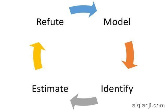
建模: DoWhy使用因果关系图来模拟每个问题。当前版本的DoWhy支持两种图形输入格式:gml(首选)和点。该图可能包括变量中因果关系的先验知识,但DoWhy没有做出任何直接的假设。
识别:使用输入图,DoWhy根据图形模型找到识别所需因果效果的所有可能方法。它使用基于图形的标准和do-calculus来找到可以找到可以识别因果效应的表达式的潜在方法
估计: DoWhy使用统计方法(如匹配或工具变量)估算因果效应。当前版本的DoWhy支持基于倾向的分层或倾向得分匹配的估计方法,这些方法侧重于估计治疗分配以及侧重于估计响应面的回归技术。
验证:最后,DoWhy使用不同的稳健性方法来验证因果效应的有效性。
Confounding Example: Finding causal effects from observed data
Suppose you are given some data with treatment and outcome. Can you determine whether the treatment causes the outcome, or the correlation is purely due to another common cause?
假设给你一些关于治疗和结果的数据。你能确定是治疗导致了结果,还是相关性纯粹是由于另一个共同的原因?
[1]:
import os, sys
sys.path.append(os.path.abspath("../../"))
[2]:
import numpy as np
import pandas as pd
import matplotlib.pyplot as plt
import seaborn as sns
import math
import dowhy
from dowhy import CausalModel
import dowhy.datasets, dowhy.plotter
Let’s create a mystery dataset for which we need to determine whether there is a causal effect. 让我们创建一个神秘的数据集,我们需要确定是否存在因果效应
Creating the dataset. It is generated from either one of two models: * Model 1: Treatment does cause outcome. * Model 2: Treatment does not cause outcome. All observed correlation is due to a common cause.
创建数据集。它产生于两种模式之一:
模式1: 治疗确实导致结果。
模式2 : 治疗不会导致结果。所有观察到的相关性都是由于一个其他共同的原因。
[3]:
rvar = 1 if np.random.uniform() >0.5 else 0
data_dict = dowhy.datasets.xy_dataset(10000, effect=rvar, sd_error=0.2)
df = data_dict['df']
print(df[["Treatment", "Outcome", "w0"]].head())
   Treatment    Outcome        w0
0   7.598026  15.812081  2.011138
1   7.601832  15.305892  1.841549
2  10.137274  19.918058  3.977756
3   9.444259  19.138840  3.790387
4   2.708849   5.403166 -3.191784
df数据如下
Treatment Outcome w0 s
0 1.869872 3.832871 -3.984799 7.123291
1 2.790359 5.671909 -3.065245 7.966827
2 2.889123 5.148204 -3.277346 7.850091
3 8.908309 17.343314 2.623172 4.173383
4 6.467875 13.052497 0.390332 9.095312
[4]:
dowhy.plotter.plot_treatment_outcome(df[data_dict["treatment_name"]], df[data_dict["outcome_name"]],
                             df[data_dict["time_val"]])

Using DoWhy to resolve the mystery: Does Treatment cause Outcome? 使用 DoWhy 来解开谜团:治疗会有效吗?
STEP 1: Model the problem as a causal graph 步骤1: 将问题建模为因果关系图
Initializing the causal model.
初始化因果模型。
[5]:
model= CausalModel(
data=df,
treatment=data_dict["treatment_name"],
outcome=data_dict["outcome_name"],
common_causes=data_dict["common_causes_names"],
instruments=data_dict["instrument_names"])
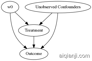
model.view_model(layout="dot")
WARNING:dowhy.causal_model:Causal Graph not provided. DoWhy will construct a graph based on data inputs.
INFO:dowhy.causal_model:Model to find the causal effect of treatment ['Treatment'] on outcome ['Outcome']
Showing the causal model stored in the local file “causal_model.png”
显示存储在本地文件“causal_model. png”中的因果模型
[6]:
from IPython.display import Image, display
display(Image(filename="causal_model.png"))
STEP 2: Identify causal effect using properties of the formal causal graph 步骤2: 使用形式因果图的属性识别因果效应
Identify the causal effect using properties of the causal graph. 使用因果图的属性来识别因果效应。
[7]:
identified_estimand = model.identify_effect()
print(identified_estimand)
INFO:dowhy.causal_identifier:Common causes of treatment and outcome:['w0', 'U']
WARNING:dowhy.causal_identifier:There are unobserved common causes. Causal effect cannot be identified.
WARN: Do you want to continue by ignoring these unobserved confounders? [y/n] y
INFO:dowhy.causal_identifier:Instrumental variables for treatment and outcome:[]
Estimand type: ate
### Estimand : 1
Estimand name: iv
No such variable found!
### Estimand : 2
Estimand name: backdoor
Estimand expression:
    d
──────────(Expectation(Outcome|w0))
dTreatment
Estimand assumption 1, Unconfoundedness: If U→Treatment and U→Outcome then P(Outcome|Treatment,w0,U) = P(Outcome|Treatment,w0)
STEP 3: Estimate the causal effect 步骤3: 估计因果效应
Once we have identified the estimand, we can use any statistical method to estimate the causal effect.
一旦我们确定了估计值,我们就可以使用任何统计方法来估计因果效应。
Let’s use Linear Regression for simplicity.
为了简单起见,让我们使用线性回归。
[8]:
estimate = model.estimate_effect(identified_estimand,
method_name="backdoor.linear_regression")
print("Causal Estimate is " + str(estimate.value))
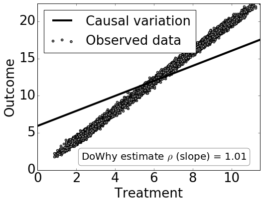
# Plot Slope of line between treamtent and outcome =causal effect
dowhy.plotter.plot_causal_effect(estimate, df[data_dict["treatment_name"]], df[data_dict["outcome_name"]])
INFO:dowhy.causal_estimator:INFO: Using Linear Regression Estimator
INFO:dowhy.causal_estimator:b: Outcome~Treatment+w0
Causal Estimate is 1.0099765763913107
Checking if the estimate is correct 检查估计是否正确
[9]:
print("DoWhy estimate is " + str(estimate.value))
print ("Actual true causal effect was {0}".format(rvar))
DoWhy estimate is 1.0099765763913107
Actual true causal effect was 1
Step 4: Refuting the estimate 第四步: 反驳这个估计
We can also refute the estimate to check its robustness to assumptions (aka sensitivity analysis, but on steroids).
我们也可以驳斥这个估计,以检验其对假设的可靠性(又名敏感度分析,但是是类固醇)。
Adding a random common cause variable 添加一个随机的公共原因变量
[10]:
res_random=model.refute_estimate(identified_estimand, estimate, method_name="random_common_cause")
print(res_random)
INFO:dowhy.causal_estimator:INFO: Using Linear Regression Estimator
INFO:dowhy.causal_estimator:b: Outcome~Treatment+w0+w_random
Refute: Add a Random Common Cause
Estimated effect:(1.0099765763913107,)
New effect:(1.009944524944634,)
Replacing treatment with a random (placebo) variable 用随机(安慰剂)变量取代治疗
[11]:
res_placebo=model.refute_estimate(identified_estimand, estimate,
        method_name="placebo_treatment_refuter", placebo_type="permute")
print(res_placebo)
INFO:dowhy.causal_estimator:INFO: Using Linear Regression Estimator
INFO:dowhy.causal_estimator:b: Outcome~placebo+w0
Refute: Use a Placebo Treatment
Estimated effect:(1.0099765763913107,)
New effect:(-0.0004315715075086384,)
Removing a random subset of the data 删除数据的随机子集
[12]:
res_subset=model.refute_estimate(identified_estimand, estimate,
        method_name="data_subset_refuter", subset_fraction=0.9)
print(res_subset)
INFO:dowhy.causal_estimator:INFO: Using Linear Regression Estimator
INFO:dowhy.causal_estimator:b: Outcome~Treatment+w0
Refute: Use a subset of data
Estimated effect:(1.0099765763913107,)
New effect:(1.007629285793896,)
As you can see, our causal estimator is robust to simple refutations.
正如你所看到的,我们的因果估计对简单的反驳是鲁棒的。
Instrumental Variable Analysis工具变量分析
IV analysis has been used for several decades in the field of econometrics to help deal with issues of confounding, reverse causality, and regression dilution bias (more often referred to collectively as “endogeneity” in econometrics) [81].
IV 分析已经在计量经济学领域使用了几十年,以帮助处理混杂、反向因果关系和回归稀释偏差(在计量经济学中通常统称为“内生性”)的问题[81]。
From: Genomic and Precision Medicine (Third Edition), 2017
摘自: 2017年《基因组与精准医学》第三版
Biostatistics Used for Clinical Investigation of Coronary Artery Disease 生物统计学在冠状动脉疾病临床调查中的应用
Chul Ahn, in Translational Research in Coronary Artery Disease, 2016
An Instrumental Variable (IV) is used to control for confounding and measurement error in observational studies so that causal inferences can be made. Suppose X and Y are the exposure and outcome of interest, and we can observe their relation to a third variable Z. Let Z be associated with X but not associated with Y except through its association with X. Here, Z is called an IV or instrument [33]. That is, an IV is a factor that is associated with the exposure but not with the outcome. For example, the price of beer can affect the likelihood of drinking beer in expectant mothers, but there is no reason to believe that it directly affects the child’s birthweight.
在观察性研究中,工具变量(IV)用于控制混杂和测量误差,以便做出因果推论。假设 x 和 y 是感兴趣的暴露和结果,我们可以观察到它们与第三个变量 z 的关系。也就是说,静脉注射是一个与暴露有关的因素,而与结果无关。例如,啤酒的价格会影响准妈妈喝啤酒的可能性,但是没有理由相信啤酒会直接影响孩子的出生体重。
Example: When surgeons show strong preference for one of the two antifibrinolytic agents, surgeon’s choice does not depend on characteristics of the patient. Then, it is possible to use the surgeon’s preferred agent as a substitute for the actual exposure (i.e., as an IV). Schneeweiss et al. [34] conducted an IV analysis to investigate the association between the use of aprotinin and death.
例如: 当外科医生表现出强烈的偏好时,外科医生的选择并不取决于病人的特点。然后,可以使用外科医生喜欢的代理人作为实际暴露的替代物(即,作为一个 IV)。Schneeweiss 等人进行了 IV 分析来调查抑肽酶的使用和死亡之间的联系。
The Microbiome in Health and Disease 健康与疾病中的微生物组
Yinglin Xia, in Progress in Molecular Biology and Translational Science, 2020
7.2.1.7.2 Redundancy analysis (RDA)冗余分析
RDA was also named as principal component analysis with instrumental variables.534 As a constrained ordination, RDA was developed to assess how much of the variation in one set of variables can be explained by the variation in another set of variables. However, as a multivariate extension of simple linear regression into sets of variables,534 RDA summarizes the linear relations between multiple dependent variables and multiple independent variables in a matrix, which is then incorporated into PCA. RDA assumes that variables from two datasets (e.g., an environmental dataset and a taxa abundance dataset) play different roles: one set of variables can be considered the “independent variables,” and the other set is considered the “dependent variables.” In other words, the variables in these two sets are asymmetrical.
作为一种约束排序,RDA 被发展用来评估一组变量的变化有多少可以被另一组变量的变化所解释。然而,作为变量集的多元简单线性回归扩展,534 RDA 总结了多个因变量和多个自变量在一个矩阵中的线性关系,然后将其纳入 PCA。RDA 假设来自两个数据集的变量(例如,一个环境数据集和一个分类数据集)扮演不同的角色: 一组变量可以被认为是“独立变量”,而另一组则被认为是“因变量”换句话说,这两个集合中的变量是不对称的。
RDA is different from canonical correlation analysis (CANCOR, also often abbreviated as CCA) in that CCA puts both sets of variables equally or treat them symmetrically. RDA has limitations such as its assumption of linear relationships among variables. RDA uses the similar principles as PCA, which is actually a canonical version of PCA where the principal components are constrained to be linear combinations of the explanatory variables. Thus, RDA is inappropriate when relationship between response and environmental variables is unimodal rather than linear. RDA was used to investigate the association between log relative abundance and different human milk consumption patterns while controlling various explanatory variables.114 Other examples of using RDA are from studies.531,535–537
RDA 不同于典型相关分析(CANCOR,也经常缩写为 CCA) ,CCA 将两组变量平等或对称地处理。RDA 有其局限性,例如它假设变量之间是线性关系。RDA 使用与 PCA 类似的原理,PCA 实际上是 PCA 的一个规范版本,其中主成分被限制为解释变量的线性组合。因此,当响应与环境变量的关系是单峰型而非线性时,RDA 是不适当的。在控制各种解释变量的同时,使用 RDA 来调查对数相对丰度和不同母乳消费模式之间的关联。114其他使用 RDA 的例子来自研究。531,535-537