因果推理3: 反事实推理（翻译）

gingo 2021-08-09 14:46:59 资料仓库收藏

0 / 805

January 24, 2019 2019年1月24日

Causal Inference 3: Counterfactuals

因果推理3: 反事实推理

Counterfactuals are weird. I wasn't going to talk about them in my MLSS lectures on Causal Inference, mainly because wasn't sure I fully understood what they were all about, let alone knowing how to explain it to others. But during the Causality Panel, David Blei made comments about about how weird counterfactuals are: how difficult they are to explain and wrap one's head around. So after that panel discussion, and with a grand total of 5 slides finished for my lecture on Thursday, I said "challenge accepted". The figures and story I'm sharing below are what I came up with after that panel discussion as I finally understood how to think about counterfactuals. I'm hoping others will find them illuminating, too.

反事实是很奇怪的。我不打算在我的因果推理的 MLSS 演讲中谈论它们，主要是因为我不确定我完全理解它们是关于什么的，更不用说知道如何向别人解释了。但是在因果小组讨论中，大卫 · 布莱评论了反事实是多么的奇怪: 要解释和理解这些事实是多么的困难。所以在那次小组讨论之后，在总共5张幻灯片完成了我周四的演讲之后，我说“接受挑战”。我在下面分享的数据和故事是我在那次小组讨论之后想出来的，因为我终于明白了如何思考反事实。我希望其他人也能从中受益。

This is the third in a series of tutorial posts on causal inference. If you're new to causal inferenece, I recommend you start from the earlier posts:

这是关于因果推理的一系列教程中的第三篇。如果你是因果推理的新手，我建议你从以前的文章开始:

Counterfactuals

反事实

Let me first point out that counterfactual is one of those overloaded words. You can use it, like Judea Pearl, to talk about a very specific definition of counterfactuals: a probablilistic answer to a "what would have happened if" question (I will give concrete examples below). Others use the terms like counterfactual machine learning or counterfactual reasoning more liberally to refer to broad sets of techniques that have anything to do with causal analysis. In this post, I am going to focus on the narrow Pearlian definition of counterfactuals. As promised, I will start with a few examples:

首先让我指出，反事实就是这些超载的词汇之一。你可以像 Judea Pearl 一样，用它来讨论反事实的一个非常具体的定义: 对“如果”问题的一个可能的答案(我将在下面给出具体的例子)。其他人则更多地使用反事实机器学习或反事实推理这样的术语来指代与因果分析有关的一系列技术。在这篇文章中，我将集中讨论狭隘的皮尔斯式的反事实定义。正如所承诺的那样，我将从几个例子开始:

Example 1: David Blei's election example

例子1: David Blei 的选举例子

This is an example David brought up during the Causality Panel and I referred back to this in my talk. I'm including it here for the benefit of those who attended my MLSS talk:

这是大卫在因果小组讨论中提到的一个例子，我在演讲中也提到了这个例子。我把它放在这里是为了那些参加我的 MLSS 演讲的人:

Given that Hilary Clinton did not win the 2016 presidential election, and given that she did not visit Michigan 3 days before the election, and given everything else we know about the circumstances of the election, what can we say about the probability of Hilary Clinton winning the election, had she visited Michigan 3 days before the election?

考虑到希拉里 · 克林顿没有赢得2016年总统大选，考虑到她没有在大选前3天访问密歇根州，考虑到我们所知道的关于大选情况的其他一切，我们对希拉里 · 克林顿赢得大选的可能性有什么可说的，她是否在大选前3天访问了密歇根州？

Let's try to unpack this. We are are interested in the probability that:

让我们来解释一下，我们感兴趣的是这种可能性:

she 她hypothetically 假设 wins the election 赢得选举

conditionied on four sets of things:

有四个条件:

she lost the election 她竞选失败了
she did not visit Michigan 她没有去密歇根
any other relevant an observable facts 任何其他相关的可观察的事实
she 她hypothetically 假设 visits Michigan 访问密歇根州

It's a weird beast: you're simultaneously conditioning on her visiting Michigan and not visiting Michigan. And you're interested in the probability of her winning the election given that she did not. WHAT?

这是一个奇怪的野兽: 你同时在她访问密歇根州和不访问密歇根州的条件反射。你对她赢得选举的可能性感兴趣，因为她没有赢。什么？

Why would quantifying this probability be useful? Mainly for credit assignment. We want to know why she lost the election, and to what degree the loss can be attributed to her failure to visit Michigan three days before the election. Quantifying this is useful, it can help political advisors make better decisions next time.

为什么量化这个概率是有用的呢？主要用于信贷转让。我们想知道她为什么在选举中落败，以及这次失败在多大程度上可以归咎于她没有在选举前三天访问密歇根州。量化这一点是有用的，它可以帮助政治顾问下次做出更好的决定。

Example 2: Counterfactual fairness

例二: 违反事实的公平性

Here's a real-world application of counterfactuals: evalueting the efairness of individual decisions. Consider this counterfactual question:

这里有一个现实世界中反事实的应用: 评估个人决策的公平性。考虑这个反事实的问题:

Given that Alice did not get promoted in her job, and given that she is a woman, and given everything else we can observe about her circumstances and performance, what is the probability of her getting a promotion if she was a man instead?

考虑到爱丽丝在工作中没有得到提升，考虑到她是一个女人，考虑到我们能观察到的关于她的情况和表现的一切，如果她是一个男人，她得到提升的可能性有多大？

Again, the main reason for asking this question is to establish to what degree being a woman is directly responsible for the observed outcome. Note that this is an individual notion of fairness, unlike the aggregate assessment of whether the promotion process is fair or unfair statistically speaking. It may be that the promotion system is pretty fair overall, but in the particular case of Alice unfair discrimination took place.

同样，提出这个问题的主要原因是为了确定作为一个女人在多大程度上对观察到的结果负有直接责任。请注意，这是一个个人的公平概念，不同于从统计学角度来看晋升过程是否公平的总体评估。总的来说，晋升制度可能是相当公平的，但在爱丽丝的个案中，不公平的歧视发生了。

A counterfactual question is about a specific datapoint, in this case Alice.

一个反事实的问题是关于一个特定的数据点，在本例中是 Alice。

Another weird thing to note about this counterfactual is that the intervention (Alice's gender magically changing to male) is not something we could ever implement or experiment with in practice.

关于这个反事实的另一个奇怪的地方是，干预(爱丽丝的性别神奇地变成了男性)并不是我们可以在实践中实施或试验的东西。

Example 3: My beard and my PhD

例子3: 我的胡子和我的博士学位

Here's the example I used in my talk, and will use throughout this post: I want to understand to what degree having a beard contributed to getting a PhD:

下面是我在演讲中使用的例子，并且将贯穿整篇文章: 我想知道留胡子对获得博士学位有多大的贡献:

Given that I have a beard, and that I have a PhD degree, and everything else we know about me, with what probability would I have obtained a PhD degree, had I never grown a beard.

考虑到我有胡子，我有博士学位，以及我们所知道的关于我的一切，如果我从来没有留过胡子，我有多大可能获得博士学位。

Before I start describing how to express this as a probability, let's first think about what we intuitively expect the answer to be? In the grand scheme of things, my beard probably was not a major contributing factor to getting a PhD. I would have pursued PhD studies, and probably completed my degree, even if something would have prevented me to keep my beard. So

在我开始描述如何将其表示为概率之前，让我们首先思考一下我们凭直觉所期望的答案是什么？从宏观的角度来看，我的胡子可能不是获得博士学位的主要影响因素。我会继续攻读博士学位，甚至可能完成我的学位，即使有些事情会阻止我留胡子。所以

We expect the answer to this counterfactual to be a high probability, something close to 1.

我们期望这个反事实的答案是一个很高的概率，接近1。

Observational queries

观察性质的询问

Let's start with the simplest thing one can do to attempt to answer my counterfactual question: collect some data about individuals, whether they have beards, whether they have PhDs, whether they are married, whether they are fit, etc. Here's a cartoon illustration of such dataset:

让我们从最简单的事情开始，试图回答我的反事实问题: 收集一些关于个人的数据，他们是否有胡子，他们是否有博士学位，他们是否已婚，他们是否健康等等。下面是这些数据的卡通插图:

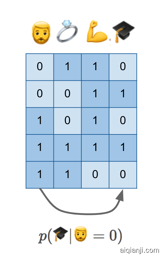
I am in this dataset, or someone just like me is in the dataset, in row number four: I have a beard, I am married, I am obviously very fit (this was the point where I hoped the audience would get the joke and laugh, and thankfully they did), and I have a PhD degree. I have it all.

我在这个数据集中，或者像我这样的人在数据集中，在第四行: 我有胡子，我结婚了，我显然非常强壮(这是我希望观众能听懂笑话并且大笑的地方，谢天谢地他们做到了) ，我有一个博士学位。我什么都有。

If we have this data and do normal statistical machine learning, without causal reasoning, we'd probably attempt to estimate p(🎓|🧔=0)p(🎓|🧔=0), the conditional probability of possessing a PhD degree given the absence of a beard. As I show at the bottom, this is like predicting values in one column from values in another column.

如果我们有这些数据，并且做正常的统计机器学习，没有因果推理，我们可能会尝试估计 p (| = 0) p (| = 0) ，因为没有胡须，所以拥有博士学位的条件概率我在底部显示，这就像从另一列中的值预测一列中的值。

You hopefully know enough about causal inference by now to know that p(🎓|🧔=0)p(🎓|🧔=0) is certainly not the quantity we seek. Without additional knowledge of causal structure, it can't generalize to hypothetical scenarios and interventions we care about her. There might be hidden confounders. Perhaps scoring high on the autism spectrum makes it more likely that you grow a beard, and it may also makes it more likely to obtain a PhD. This conditional isn't aware if the two quantities are causally related or not.

希望您现在已经足够了解因果推理，知道 p (| = 0) p (| = 0)肯定不是我们要求的量虽然有关因果结构的额外知识，它不能概括到我们所关心的假设情景和干预可能有隐藏的混淆因素也许在自闭症谱系中得分较高会使你更有可能留胡子，也可能使你更有可能获得博士学位不知道这两个量是否有因果关系。

Intervention queries

干预查询

We've learned in the previous two posts that if we want to reason about interventions, we have to express a different conditional distribution, p(🎓|do(🧔=0))p(🎓|do(🧔=0)). We also know that in order to reason about this distribution, we need more than just a dataset, we also need a causal diagram. Let's add a few things to our figure:

我们在前两篇文章中已经了解到，如果我们想要推理干预，我们必须表达一个不同的条件分布，p (| do (= 0)) p (| do (= 0))也知道，为了推理这种分布，我们需要的不仅仅是一个数据集，我们还需要一个因果图我们再加上几点:

Here, I drew a cartoon causal diagram on top of the data just for illustration, it was simply copy-pasted from previous figures, and does not represent a grand unifying theory of beards and PhD degrees. But let's assume our causal diagram describes reality.

在这里，我在数据上面画了一个卡通因果关系图，只是为了说明问题，它只是从以前的数据中复制粘贴出来的，并不代表胡须和博士学位的宏大统一理论。但是让我们假设我们的因果关系图描述了现实。

The causal diagram lets us reason about the distribution of data in an alternative world, a parallel universe if you like, in which everyone is somehow magically prevented to grow a beard. You can imagine sampling a dataset from this distribution, shown in the green table. We can measure the association between PhD degrees and beards in this green distribution, which is precisely what p(🎓|do(🧔=0))p(🎓|do(🧔=0)) means. As shown by the arrow below the tables, p(🎓|do(🧔=0))p(🎓|do(🧔=0)) is about predicting columns of the green dataset from other columns of the green dataset.

因果关系图让我们可以推理数据在另一个世界中的分布情况，如果你愿意的话，这是一个平行宇宙，在这个世界中，每个人都奇迹般地避免了留胡子。您可以想象从这个分布中取样数据集，如绿表所示。我们可以在这个绿色分布中测量博士学位和胡子之间的关系，这正是 p (| do (= 0)) p (| do (= 0))的意思通过表下方的箭头显示，p (| do (= 0)) p (| do (= 0))是关于从绿色数据集的其他列预测绿色数据集的列。

Can p(🎓|do(🧔=0))p(🎓|do(🧔=0)) express the counterfactual probability we seek? Well, remember that we expected that I would have obtained a PhD degree with a high probability even without a beard. However, p(🎓|do(🧔=0))p(🎓|do(🧔=0)) talks about a the PhD of a random individual after a no-beard intervention. If you take a random person off the street, shave their beard if they have one, it is not very likely that your intervention will cause them to get a PhD with a high probability. Not to mention that your intervention has no effect on most women and men without beards. We intuitively expect p(🎓|do(🧔=0))p(🎓|do(🧔=0)) to be close to the base-rate of PhD degrees p(🎓)p(🎓), which is apparently somewhere around 1-3%.

P (| do (= 0)) p (| do (= 0))能表达我们所寻求的反事实概率吗别忘了，我们以为即使没有胡子，我也很有可能获得博士学位不管怎样，p (| do (= 0)) p (| do (= 0)谈论的是一个随机的个体在没有胡子的干预后的哲学博士如果你在街上随便抓一个人，如果他们有胡子的话就剃掉他们的胡子，你的干预不太可能使他们获得高概率的博士学位你的介入对大多数没有胡须的男女没有任何影响本质上期望 p (| do (= 0)) p (| do (= 0))接近于哲学博士学位 p () p ()的基本概率，显然在1-3% 左右。

p(🎓|do(🧔=0))p(🎓|do(🧔=0)) talks about a randomly sampled individual, while a counterfactual talks about a specific individual

P (| do (= 0)) p (| do (= 0))谈论一个随机抽样的个体，而一个反事实的谈论一个特定的个体

Counterfactuals are "personalized" in the sense that you'd expect the answer to change if you substitute a different person in there. My father has a mustache, (let's classify that as a type of beard for pedagogical purposes), but he does not have a PhD degree. I expect that preventing him to grow a mustache would not have made him any more likely to obtain a PhD. So his counterfactual probability would be a probability close to 0.

反事实是“个性化的”，因为如果你在其中替换一个不同的人，你会期望答案发生改变。我父亲有胡子，(我们把它归类为一种教学用的胡子) ，但是他没有博士学位。我希望阻止他留胡子不会使他更有可能获得博士学位。所以他的反事实概率接近于0。

The counterfactual probabilities vary from person to person. If you calculate them for random individuals, and average the probabilities, you should expect to to get something like p(🎓|do(🧔=0))p(🎓|do(🧔=0)) in expectation. (More on this connection later.) But we not interested in the population mean now, but are interested in calculating the probabilities for each individual.

反事实的概率因人而异。如果你为随机个体计算它们，然后平均概率，你应该期望得到像 p (| do (= 0)) p (| do (= 0))这样的期望值B) b)【句意】这条线路是我们以后的交通枢纽我们对现在的人口平均数不感兴趣，而是对计算每个人的概率感兴趣。

Counterfactual queries

反事实质疑

To finally explain counterfactuals, I have to step beyond causal graphs and introduce another concept: structural equation models.

为了最终解释反事实，我必须超越因果图，引入另一个概念: 结构方程模型。

Structural Equation Models

结构方程模型

A causal graph encodes which variables have a direct causal effect on any given node - we call these causal parents of the node. A structural equation model goes one step further to specify this dependence more explicitly: for each variable it has a function which describes the precise relationship between the value of each node the value of its causal parents.

一个因果图对变量进行编码，这些变量对任何给定的节点都有直接的因果影响——我们称这些节点的因果父节点。结构方程模型更进一步，更明确地说明了这种依赖性: 对于每个变量，它都有一个函数，该函数描述了每个节点的值与其因果父母的值之间的精确关系。

It's easiest to illustrate this through an example: here's a causal graph of an online advertising system, taken from the excellent paper of Bottou et al, (2013):

通过一个例子最容易说明这一点: 这是一个在线广告系统的因果关系图，摘自 Bottou et al (2013)的优秀论文:

It doesn't really matter what these variables mean, if interested, read the paper. The dependencies shown by the diagram are equivalently encoded by the following set of equations:

这些变量意味着什么并不重要，如果你感兴趣的话，读读报纸吧。图中显示的依赖关系等价地由以下方程组编码:

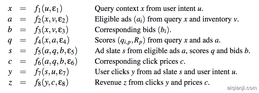
For each node in the graph above we now have a corresponding function fifi. The arguments of each function are the causal parents of the variable it instantiates, e.g. f1f1 computes xx from its causal parent uu, and f2f2 computes aa from its causal parents xx and vv. In order to allow for nondeterministic relationship between the variables, we additionally allow each function fifi to take another input, ϵiϵi which you can think of as a random number. Through the random input ϵ1ϵ1, the output of f1f1 can be random given a fixed value of uu, hence giving rise to a conditional distribution p(x|u)p(x|u).

对于上图中的每个节点，我们现在都有一个相应的函数 f i fi。每个函数的参数是它实例化的变量的因果父变量，例如 f1 f1从它的因果父变量 u 计算 x，f2 f2从它的因果父变量 x 和 v 计算 a。为了考虑变量之间的不确定关系，我们另外允许每个函数 f i fi 采用另一个输入，你可以把它看作是一个随机数。通过随机输入 ε1ε1，f1f1的输出可以随机给定一个固定的 u 值，从而产生一个条件分布 p (x | u) p (x | u)。

The structural equation model (SEM) entails the causal graph, in that you can reconstruct the causal graph by looking at the inputs of each function. It also entails the joint distribution, in that you can "sample" from an SEM by evaluating the functions in order, plugging in the random ϵϵs where needed.

结构方程模型(SEM)包含了因果图，因为您可以通过查看每个函数的输入来重建因果图。它还需要联合分布，即你可以通过按顺序评估函数从 SEM 中“取样”，在需要的地方插入随机 ε s。

In a SEM an intervention on a variable, say qq, can be modelled by deleting the corresponding function, f4f4, and replacing it with another function. For example do(Q=q0)do(Q=q0) would correspond to a simple assignment to a constant f~4(x,a)=q0f~4(x,a)=q0.

在 SEM 中，可以通过删除对应的函数 f4f4，然后用另一个函数替换来模拟对一个变量的干预，比如 q。例如 do (q = q0) do (q = q0)对应于一个常数 f ~ 4(x，a) = q0 f ~ 4(x，a) = q0的简单赋值。

Back to the beard example

回到胡子的例子

Now that we know what SEMs are we can return to our example of beards and degrees. Let's add a few more things to the figure:

现在我们知道了什么是小型企业，我们可以回到我们的胡子和学位的例子。让我们在这个数字上再加上一些东西:

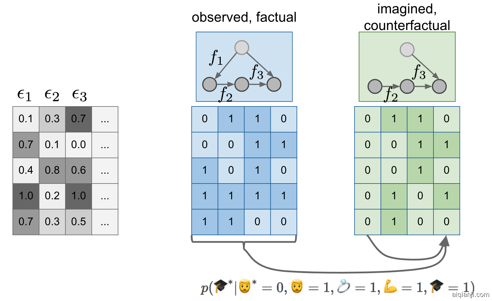
First change is, that instead of just a causal graph, I now assume that we model the world by a fully specified structural equation model. I signify this lazily by labelling the causal graph with the functions f1,f2,f3f1,f2,f3 over the graph. Notice that the SEM of the green situation is the same as the SEM in the blue case, except that I deleted f1f1 and replaced it with a constant assignment. But f2f2 and f3f3 are the same between the blue and the green models.

第一个变化是，我现在假设我们用一个完全指定的结构方程模型，来模拟这个世界，而不仅仅是一个因果图。我懒洋洋地用图上的函数 f1，f2，f3 f1，f2，f3来表示这个因果图。注意，绿色情况下的 SEM 与蓝色情况下的 SEM 相同，只是我删除了 f1 f1并用一个常量赋值代替了它。但是 f2f2和 f3f3在蓝色模型和绿色模型中是相同的。

Secondly, I make the existence of the ϵiϵi noise variables explicit, and show their values (it's all made up of course) in the gray table. If you feed the first row of epsilons to the blue structural equation model, you get the first blue datapoint 01100110. If you feed the same epsilons to the green SEM, you get the first green datapoint (0110)(0110). If you feed the second row of epsilons to the models, you get the second rows in the blue and green tables, and so on...

其次，明确了 ε i εi 噪声变量的存在性，并在灰度表中显示它们的值(当然都是由它们组成的)。如果将第一行 epsilon 提供给 blue 结构方程模型，就会得到第一个蓝色数据点01100110。如果您将相同的 epsilon 提供给绿色 SEM，您将获得第一个绿色数据点(0110)(0110)。如果将第二行 epsilon 提供给模型，则会得到蓝色和绿色表中的第二行，依此类推..。

I like to think about the first green datapoint as the parallel twin of the first blue datapoint. To talk about interventions I talked about this making predictions about a parallel universe where nobody has a beard. Now imagine that for every person who lives in our observable universe, there is a corresponding person, their parallel twin, in this parallel universe. Your twin is same in every respect as you, except for the absence of any beard you might have and any downstream consequences of having a beard. If you don't have a beard in this universe, your twin is an exact copy of you in every respect. Indeed, notice that the first blue datapoint is the same as the first green datapoint in my example.

我喜欢把第一个绿色数据点想象成与第一个蓝色数据点平行的双胞胎。在谈到干预时，我谈到了这种对平行宇宙的预测，在这个宇宙中没有人留胡子。现在想象一下，对于每一个生活在我们可观测宇宙的人，在这个平行宇宙中都有一个对应的人，他们的平行孪生兄弟。你的双胞胎兄弟和你在各个方面都是一样的，除了你可能没有胡子，以及你有胡子的下游后果。如果你在这个宇宙中没有胡子，那么你的双胞胎兄弟在各个方面都是你的一模一样。实际上，请注意，第一个蓝色数据点与我的示例中的第一个绿色数据点相同。

You may know I'm a Star Trek fan and I like to use Star Trek analogies to explain things: In Star Trek, there is this concept called the mirror universe. It's a parallel universe populated by the same people who live in the normal universe, except that everyone who is good in the real universe is evil in the mirror universe. Hilariously, the mirror version of Spock, one of the main protagonists, has a goatie in this mirror universe. This is how you could tell if you're looking at evil mirror-Spock or normal Spock when watching the episode. This explains, sadly, why I'm using beards to explain counterfactuals. Here are Spock and mirror-Spock:

你可能知道我是《星际迷航》的粉丝，我喜欢用《星际迷航》的类比来解释一些事情: 在《星际迷航》中，有一个概念叫做镜像宇宙。这是一个平行宇宙，由生活在正常宇宙中的同一批人组成，只不过现实宇宙中的每一个好人在镜像宇宙中都是邪恶的。滑稽的是，镜像版的斯波克，主角之一，在这个镜像宇宙中有一个羔羊。这就是你在观看这一集的时候，如果你看到的是邪恶的镜子——史波克或者正常的史波克。不幸的是，这解释了为什么我要用胡子来解释反事实。这是斯波克和镜子斯波克:

Now that we established the twin datapoint metaphor, we can say that counterfactuals are

既然我们已经建立了双数据点隐喻，我们可以说反事实是

making a prediction about features of the unobserved twin datapoint based on features of the observed datapoint.

根据观测数据点的特征对未观测到的双数据点特征进行预测。

Crucially, this was possible because we used the same ϵϵs in both the blue and the green SEM. This induces a joint distribution between variables in the observable regime, and variables in the unobserved, counterfactual regime. Columns of the green table are no longer independent of columns of the blue table. You can start predicting values in the green table using values in the blue table, as illustrated by the arrows below them.

至关重要的是，这是可能的，因为我们在蓝色和绿色扫描电镜中使用了相同的 ε s。这就导致了可观察状态下的变量和不可观察的反事实状态下的变量之间的联合分布。绿表的列不再独立于蓝表的列。您可以开始使用蓝色表格中的值来预测绿色表格中的值，如下面的箭头所示。

Mathematically, a counterfactual is the following conditional probability:

数学上，一个反事实的条件概率是:

p(🎓∗|🧔∗=0,🧔=1,💍=1,💪=1,🎓=1)

第一次 * * * * * * * * * * * * * * * * * * * * ,

where variables with an ∗∗ are unobserved (and unobservable) variables that live in the counterfactual world, while variables without ∗∗ are observable.

- - - - .

Looking at the data, it turns out that mirror-Ferenc, who does not have a beard, is married and has PhD, but is not quite as strong as observable Ferenc.

从数据来看，镜子-费伦茨，没有胡子，已婚，有博士学位，但是没有可观察到的费伦茨那么强壮。

Another way to draw this

另一种方法来描述这个

Here is another drawing that some of you might find more appealing, especially those who are are into GANs, VAEs and similar generative models:

下面是另一幅图，你们中的一些人可能会觉得更有吸引力，特别是那些喜欢 GANs，VAEs 和类似的生成模型的人:

A SEM is essentially a generative model of data, which uses some noise variables ϵ1,ϵ2,…ϵ1,ϵ2,… and turns them into observations (U,Z,X,Y)(U,Z,X,Y) in this example. This is shown in the left-hand branch of the graph above. Now if you want to make counterfactual statements under the intervention X=x^X=x^, you can construct a *mutilated* SEM, which is the same SEM except with f3f3 deleted and replaced with the constant assignment x=x^x=x^. This modified SEM is shown in the right-hand branch. If you feed the ϵϵs into the mutilated SEM, you get another set of variables (U∗,Z∗,X∗,Y∗)(U∗,Z∗,X∗,Y∗), shown in green. These are the features of the twin as it were. This joint generative model over (U,Z,X,Y)(U,Z,X,Y) and (U∗,Z∗,X∗,Y∗)(U∗,Z∗,X∗,Y∗) defines a joint distribution over the combined set of variables (U,Z,X,Y,U∗,Z∗,X∗,Y∗)(U,Z,X,Y,U∗,Z∗,X∗,Y∗). Therefore, now you can calculate all sorts of conditionals and marginals of this joint.

扫描电子显微镜本质上是一个生成模型的数据，它使用一些噪声变量 ε1，ε2，... ε1，ε2，... 并将它们转化为本例中的观测值(u，z，x，y)(u，z，x，y)。这在上图的左边分支中显示出来。现在，如果你想在干预 x = x ^ x = x ^ 的情况下做出反事实陈述，你可以构造一个残缺的 SEM，它与之前的 SEM 相同，只是删除了 f 3 f 3，代之以常数赋值 x = x ^ x = x ^ 。改进后的扫描电子显微镜(SEM)显示在右侧分支上。如果你把 ε s 放入残缺不全的扫描电子显微镜，你会得到另外一组变量(u/* 、 z/* 、 x/* 、 y/)(u/ 、 z/* 、 x/* 、 y/*) ，绿色显示。这就是这对孪生兄弟的特征。(u/x x y)(u/x x x x x x y)和(u/x x x x x x x x x x x x x x x x x * *)(u/x x x x x x x x x x x x x * * *)(u/x x x x x x x x x * * * * *)(u，z/x x x x x x x x x x * * * * * * * * * * * * * * * * * * * * * * * * * * * * * * * * * * * * * * * * * * * * * * * * * * * * * * * * * * * * * * * * * * * * * * * * * * * * * * * * * * * * * * * * * * * * * * * * * * * * * * * * * * * * *)。因此，现在您可以计算这个联合的所有条件和边缘。

Of particular interest are these conditionals:

特别感兴趣的是这些条件句:

p(y∗|X∗=x^,X=x,Y=y,U=u,Z=z),p(y∗|X∗=x^,X=x,Y=y,U=u,Z=z),

p (y * | x * = x ^ ，x = x，y = y，u = u，z = z) ，p (y * | x * = x ^ ，x = x，y = y，u = u，z = z) ,

which is a counterfactual prediction. In reality, since X∗=x^X∗=x^ holds with a probability of 11, we can drop that conditioning.

这是一个反事实的预言。事实上，由于 x * = x ^ x * = x ^ 的概率为1/1，我们可以放弃这种条件作用。

My notation here is a bit sloppy, there are a lot of things going on implicitly under the hood, which I'm not making explicit in the notation. I'm sorry if it causes any irritation to people, I want to avoid overcomplicating things at this point. Now is a good time to point out that Pearl's notation, including do-notation is often criticized, but people use it because now it's widely adopted.

我在这里的注释有点草率，有很多事情隐藏在背后，我没有在注释中明确说明。我很抱歉，如果它引起任何人的愤怒，我想避免过度复杂的事情在这一点上。现在是指出 Pearl 的符号(包括 do-notation)经常受到批评的好时机，但人们使用它是因为现在它被广泛采用了。

We can also express the intervention conditional p(y|do(x))p(y|do(x)) using this (somewhat sloppy) notation as:

我们也可以用这个(有点草率的)符号来表示干预条件 p (y | do (x))) p (y | do (x)) :

p(y|do(X=x^))=p(y∗|X∗=x^)p(y|do(X=x^))=p(y∗|X∗=x^)

P (y | do (x = x ^) = p (y x x x x x x x x x x x ^) p (y | do (x = x ^)) = p (y x x x x x x x x x x ^)

We can see that the intervention conditional only contains variables with an ∗∗ so it does not require the joint distribution of (U,Z,X,Y,U∗,Z∗,X∗,Y∗)(U,Z,X,Y,U∗,Z∗,X∗,Y∗) only the marginal of the ∗∗ variables (X∗,Z∗,X∗,Y∗)(X∗,Z∗,X∗,Y∗). As a consequence in order to talk about p(y|do(X=x^))p(y|do(X=x^)) we did not need to introduce SEMs or talk about the epsilons.

我们可以看到，有条件的介入次数只包含有 * * 次数的变数，因此不需要(u，z，x，y，u/* ，z/* ，x/* ，y/* ，u///* / * * * * * * * * * * * * * * * * * * * * * * * * * * * * * * * * * * * * * * * * * * * * * * * * * * * * * * * * * * * * * * * * * * * * * * * * * * * * * * * * * * * * * * * * * * * * * * * * * * * * * * * * * * * * * * * * * * * * * * * * * * * * * * * * * * * * * *。因此，为了讨论 p (y | do (x = x ^)) p (y | do (x = x ^)) ，我们不需要引入 SEMs 或讨论 epsilon。

Furthermore, notice the following equality:

此外，请注意下面的等式:

句子太长，请提供一个短句,

in other words, the intervention conditional p(y|do(X=x^))p(y|do(X=x^)) is the average of counterfactuals over the obserevable population. This was something that I did did not realize before my MLSS tutorial, and it was pointed out to me by a student in the form of a question. In hindsight, of course this is true!

换句话说，干预条件 p (y | do (x = x ^)) p (y | do (x = x ^))是可观察总体上反事实的平均值。这是我没有意识到之前，我的 MLSS 教程，它是指出给我的学生在一个问题的形式。事后看来，这当然是真的！

Summary

摘要

God, this was a loooong post. If you're still reading, thanks, I hope it was useful. I wanted to close with a few slightly philosophical remarks on counterfactuals.

天啊，这是一个很长的柱子。如果你还在读的话，谢谢，我希望这对你有帮助。我想以一些关于反事实的略带哲学色彩的评论来结束我的演讲。

Counterfactuals are often said to be unscientific, primarily because they are not empirically testable. In normal ML we are used to benchmark datasets, and that the quality of our predictions can always be tested on some test dataset. In causal ML, not everything can be directly tested or empirically benchmarked. For interventions, the best test is to run a randomized controlled trial to directly measure p(y|do(X=x))p(y|do(X=x)) if you can, and then use this experiemental data to evaluate your causal inferences. But some interventions are impossible to carry out in practice. Think about all the work on fairness reasoning about interventions on gender or race. So what to do then?

反事实常常被认为是不科学的，主要是因为它们不能经验验证。在正常的机器学习中，我们习惯于对数据集进行基准测试，并且我们的预测的质量总是可以在一些测试数据集上进行测试。在因果的机器学习中，并不是所有的东西都可以被直接测试或者基准测试。对于干预，最好的测试方法是运行一个随机对照试验，如果可能的话，直接测量 p (y | do (x = x)) p (y | do (x = x)) ，然后使用这些经验数据来评估你的因果推论。但有些干预措施在实践中是不可能实施的。想想所有关于性别或种族干预的公平推理的工作。那么接下来该怎么办呢？

In the world of counterfactuals this is an even bigger problem, as it is outright impossible to observe the variables you make predictions about. You can't go back in time and rerun history with exactly the same circumstances except for a tiny change. You can't travel to parallel universes (at least not before the 24th century, according to Star Trek). Counterfactual judgments remain hypothetical, subjective, untestable, unfalsifiable. There can be no MNIST or Imagenet for counterfactuals that satisfies everyone, though some good datasets exist, they are for specific scenarios where explicit testing is possible (e.g. offline A/B testing), or make use of simulators instead of "real" data.

在反事实的世界里，这是一个更大的问题，因为完全不可能观察到你做出预测的变量。你不可能回到过去，在完全相同的情况下重新运行历史，除了一个微小的变化。你不能到平行宇宙去旅行(至少在24世纪之前不能，根据《星际迷航》的说法)。反事实判断依然是假设性的、主观的、不可测试的、不可证伪的。尽管存在一些优秀的数据集，但是对于可以进行显式测试(如脱机 a/b 测试)的特定场景，或者使用模拟器而不是“真实”数据的场景，不可能存在能够满足所有人的虚拟事实的 MNIST 或 imageet。

Despite it being untestable, and difficult to interpret, humans make use of counterfactual statements all the time, and intuitively it feels like they are pretty useful for intelligent behaviour. Being able to pinpoint the causes that lead to a particular situation or outcome is certainly useful for learning, reasoning and intelligence. So my strategy for now is to ignore the philosophical debate about counterfactuals, and just get on with it, knowing that the tools are there if such predictions have to be made.

尽管它是不可测试的，也很难解释，但是人类一直在使用反事实的陈述，而且直觉上感觉它们对于智能行为是非常有用的。能够确定导致特定情况或结果的原因对于学习、推理和智力肯定是有用的。因此，我目前的策略是忽略关于反事实的哲学辩论，只管继续下去，知道如果必须做出这样的预测，工具就在那里。
https://www.inference.vc/causal-inference-3-counterfactuals/