D-FINE: REDEFINE REGRESSION TASK IN DETRS AS FINE-GRAINED DISTRIBUTION REFINEMENT
D-FINE:将DETR中的回归任务重新定义为细粒度分布优化

Figure 1: Comparisons with other detectors in terms of latency (left), model size (mid), and computational cost (right). We measure end-to-end latency using TensorRT FP16 on an NVIDIA T4 GPU.
图 1: 与其他检测器在延迟(左)、模型大小(中)和计算成本(右)方面的比较。我们在 NVIDIA T4 GPU 上使用 TensorRT FP16 测量端到端延迟。
ABSTRACT
摘要
We introduce D-FINE, a powerful real-time object detector that achieves outstanding localization precision by redefining the bounding box regression task in DETR models. D-FINE comprises two key components: Fine-grained Distribution Refinement (FDR) and Global Optimal Localization Self-Distillation (GO-LSD). FDR transforms the regression process from predicting fixed coordinates to iterative ly refining probability distributions, providing a fine-grained intermediate representation that significantly enhances localization accuracy. GOLSD is a bidirectional optimization strategy that transfers localization knowledge from refined distributions to shallower layers through self-distillation, while also simplifying the residual prediction tasks for deeper layers. Additionally, D-FINE incorporates lightweight optimization s in computationally intensive modules and operations, achieving a better balance between speed and accuracy. Specifically, D-FINE-L / X achieves $54.0%/55.8%$ AP on the COCO dataset at 124 / 78 FPS on an NVIDIA T4 GPU. When pretrained on Objects365, D-FINE-L / X attains $57.1%/59.3%$ AP, surpassing all existing real-time detectors. Furthermore, our method significantly enhances the performance of a wide range of DETR models by up to $5.3%$ AP with negligible extra parameters and training costs. Our code and pretrained models: https://github.com/Peterande/D-FINE.
我们介绍了 D-FINE,这是一种强大的实时目标检测器,通过重新定义 DETR 模型中的边界框回归任务,实现了出色的定位精度。D-FINE 包含两个关键组件:细粒度分布优化 (Fine-grained Distribution Refinement, FDR) 和全局最优定位自蒸馏 (Global Optimal Localization Self-Distillation, GO-LSD)。FDR 将回归过程从预测固定坐标转变为迭代优化概率分布,提供了细粒度的中间表示,显著提高了定位精度。GO-LSD 是一种双向优化策略,通过自蒸馏将定位知识从优化后的分布传递到较浅层,同时简化了较深层的残差预测任务。此外,D-FINE 在计算密集型模块和操作中引入了轻量级优化,在速度和精度之间实现了更好的平衡。具体来说,D-FINE-L/X 在 NVIDIA T4 GPU 上以 124/78 FPS 的速度在 COCO 数据集上实现了 $54.0%/55.8%$ AP。在 Objects365 上预训练后,D-FINE-L/X 达到了 $57.1%/59.3%$ AP,超越了所有现有的实时检测器。此外,我们的方法显著提升了多种 DETR 模型的性能,AP 提升了高达 $5.3%$,且额外参数和训练成本几乎可以忽略不计。我们的代码和预训练模型:https://github.com/Peterande/D-FINE。
1 INTRODUCTION
1 引言
The demand for real-time object detection has been increasing across various applications (Arani et al., 2022). Among the most influential real-time detectors are the YOLO series (Redmon et al., 2016a; Wang et al., 2023a;b; Glenn., 2023; Wang & Liao, 2024; Wang et al., 2024a; Glenn., 2024), widely recognized for their efficiency and robust community ecosystem. As a strong competitor, the Detection Transformer (DETR) (Carion et al., 2020; Zhu et al., 2020; Liu et al., 2021; Li et al., 2022; Zhang et al., 2022) offers distinct advantages due to its transformer-based architecture, which allows for global context modeling and direct set prediction without reliance on Non-Maximum Suppression (NMS) and anchor boxes. However, they are often hindered by high latency and computational demands (Zhu et al., 2020; Liu et al., 2021; Li et al., 2022; Zhang et al., 2022). RT-DETR (Zhao et al., 2024) addresses these limitations by developing a real-time variant, offering an end-to-end alternative to YOLO detectors. Moreover, LW-DETR (Chen et al., 2024) has shown that DETR can achieve higher performance ceilings than YOLO, especially when trained on large-scale datasets like Objects365 (Shao et al., 2019).
实时目标检测的需求在各种应用中不断增加 (Arani et al., 2022)。其中最具影响力的实时检测器是YOLO系列 (Redmon et al., 2016a; Wang et al., 2023a;b; Glenn., 2023; Wang & Liao, 2024; Wang et al., 2024a; Glenn., 2024),因其效率和强大的社区生态系统而广受认可。作为强有力的竞争对手,Detection Transformer (DETR) (Carion et al., 2020; Zhu et al., 2020; Liu et al., 2021; Li et al., 2022; Zhang et al., 2022) 凭借其基于Transformer的架构,提供了独特的优势,能够进行全局上下文建模,并且无需依赖非极大值抑制 (NMS) 和锚框即可直接进行集合预测。然而,它们往往受到高延迟和高计算需求的限制 (Zhu et al., 2020; Liu et al., 2021; Li et al., 2022; Zhang et al., 2022)。RT-DETR (Zhao et al., 2024) 通过开发实时变体解决了这些限制,为YOLO检测器提供了一种端到端的替代方案。此外,LW-DETR (Chen et al., 2024) 表明,DETR在诸如Objects365 (Shao et al., 2019) 等大规模数据集上训练时,可以比YOLO达到更高的性能上限。
Despite the substantial progress made in real-time object detection, several unresolved issues continue to limit the performance of detectors. One key challenge is the formulation of bounding box regression. Most detectors predict bounding boxes by regressing fixed coordinates, treating edges as precise values modeled by Dirac delta distributions (Liu et al., 2016; Ren et al., 2015; Tian et al., 2019; Lyu et al., 2022). While straightforward, this approach fails to model localization uncertainty. Consequently, models are constrained to use L1 loss and IoU loss, which provide insufficient guidance for adjusting each edge independently (Girshick, 2015). This makes the optimization process sensitive to small coordinate changes, leading to slow convergence and suboptimal performance. Although methods like GFocal (Li et al., 2020; 2021) address uncertainty through probability distributions, they remain limited by anchor dependency, coarse localization, and lack of iterative refinement. Another challenge lies in maximizing the efficiency of real-time detectors, which are constrained by limited computation and parameter budgets to maintain speed. Knowledge distillation (KD) is a promising solution, transferring knowledge from larger teachers to smaller students to improve performance without increasing costs (Hinton et al., 2015). However, traditional KD methods like Logit Mimicking and Feature Imitation have proven inefficient for detection tasks and can even cause performance drops in state-of-the-art models (Zheng et al., 2022). In contrast, localization distillation (LD) has shown better results for detection. Nevertheless, integrating LD remains challenging due to its substantial training overhead and incompatibility with anchor-free detectors.
尽管实时目标检测取得了显著进展,但一些未解决的问题仍然限制了检测器的性能。一个关键挑战是边界框回归的公式化。大多数检测器通过回归固定坐标来预测边界框,将边缘视为由狄拉克δ分布建模的精确值 (Liu et al., 2016; Ren et al., 2015; Tian et al., 2019; Lyu et al., 2022)。虽然这种方法简单直接,但未能建模定位不确定性。因此,模型被限制使用L1损失和IoU损失,这些损失无法为独立调整每个边缘提供足够的指导 (Girshick, 2015)。这使得优化过程对小的坐标变化敏感,导致收敛速度慢和性能不佳。尽管像GFocal (Li et al., 2020; 2021) 这样的方法通过概率分布解决了不确定性问题,但它们仍然受限于锚点依赖、粗略定位以及缺乏迭代优化。另一个挑战在于最大化实时检测器的效率,这些检测器受限于有限的计算和参数预算以保持速度。知识蒸馏 (Knowledge Distillation, KD) 是一种有前途的解决方案,它将知识从较大的教师模型转移到较小的学生模型,从而在不增加成本的情况下提高性能 (Hinton et al., 2015)。然而,传统的KD方法如Logit Mimicking和Feature Imitation在检测任务中已被证明效率低下,甚至可能导致最先进模型的性能下降 (Zheng et al., 2022)。相比之下,定位蒸馏 (Localization Distillation, LD) 在检测中表现出更好的效果。然而,由于LD的训练开销较大且与无锚点检测器不兼容,其集成仍然具有挑战性。
To address these issues, we propose D-FINE, a novel real-time object detector that redefines bounding box regression and introduces an effective self-distillation strategy. Our approach tackles the problems of difficult optimization in fixed-coordinate regression, the inability to model localization uncertainty, and the need for effective distillation with less training cost. We introduce Finegrained Distribution Refinement (FDR) to transform bounding box regression from predicting fixed coordinates to modeling probability distributions, providing a more fine-grained intermediate representation. FDR refines these distributions iterative ly in a residual manner, allowing for progressively finer adjustments and improving localization precision. Recognizing that deeper layers produce more accurate predictions by capturing richer localization information within their probability distributions, we introduce Global Optimal Localization Self-Distillation (GO-LSD). GO-LSD transfers localization knowledge from deeper layers to shallower ones with negligible extra training cost. By aligning shallower layers’ predictions with refined outputs from later layers, the model learns to produce better early adjustments, accelerating convergence and improving overall performance. Furthermore, we streamline computationally intensive modules and operations in existing real-time DETR architectures (Zhao et al., 2024; Chen et al., 2024), making D-FINE faster and more lightweight. While such modifications typically result in performance loss, FDR and GO-LSD effectively mitigate this degradation, achieving a better balance between speed and accuracy.
为了解决这些问题,我们提出了 D-FINE,一种新颖的实时目标检测器,它重新定义了边界框回归,并引入了一种有效的自蒸馏策略。我们的方法解决了固定坐标回归中优化困难、无法建模定位不确定性以及需要以更低的训练成本进行有效蒸馏的问题。我们引入了细粒度分布精炼 (FDR) ,将边界框回归从预测固定坐标转变为建模概率分布,提供了更细粒度的中间表示。FDR 以残差的方式迭代地精炼这些分布,允许逐步进行更精细的调整并提高定位精度。我们认识到,更深层次通过在其概率分布中捕获更丰富的定位信息来产生更准确的预测,因此我们引入了全局最优定位自蒸馏 (GO-LSD) 。GO-LSD 以几乎可以忽略的额外训练成本将定位知识从更深层次传递到更浅层次。通过将更浅层次的预测与后续层次的精炼输出对齐,模型学会产生更好的早期调整,加速收敛并提高整体性能。此外,我们简化了现有实时 DETR 架构 (Zhao et al., 2024; Chen et al., 2024) 中计算密集型的模块和操作,使 D-FINE 更快且更轻量。虽然此类修改通常会导致性能下降,但 FDR 和 GO-LSD 有效地缓解了这种退化,在速度和准确性之间实现了更好的平衡。
Experimental results on the COCO dataset (Lin et al., 2014a) demonstrate that D-FINE achieves state-of-the-art performance in real-time object detection, surpassing existing models in accuracy and efficiency. D-FINE-L and D-FINE-X achieve $54.0%$ and $55.8%$ AP, respectively on COCO val2017, running at $124;\mathrm{FPS}$ and 78 FPS on an NVIDIA T4 GPU. After pre training on larger datasets like Objects365 (Shao et al., 2019), the D-FINE series attains up to $59.3%$ AP, surpassing all existing real-time detectors, showcasing both s cal ability and robustness. Moreover, our method enhances a variety of DETR models by up to $5.3%$ AP with negligible extra parameters and training costs, demonstrating its flexibility and general iz ability. In conclusion, D-FINE pushes the performance boundaries of real-time detectors. By addressing key challenges in bounding box regression and distillation efficiency through FDR and GO-LSD, we offer a meaningful step forward in object detection, inspiring further exploration in the field.
在COCO数据集(Lin et al., 2014a)上的实验结果表明,D-FINE在实时目标检测中实现了最先进的性能,在准确性和效率方面超越了现有模型。D-FINE-L和D-FINE-X在COCO val2017上分别达到了$54.0%$和$55.8%$的AP(平均精度),在NVIDIA T4 GPU上分别以$124;\mathrm{FPS}$和78 FPS的速度运行。在更大的数据集(如Objects365(Shao et al., 2019))上进行预训练后,D-FINE系列的AP达到了$59.3%$,超越了所有现有的实时检测器,展示了其可扩展性和鲁棒性。此外,我们的方法通过FDR和GO-LSD解决了边界框回归和蒸馏效率的关键挑战,使各种DETR模型的AP提高了$5.3%$,而额外的参数和训练成本几乎可以忽略不计,展示了其灵活性和通用性。总之,D-FINE推动了实时检测器的性能边界,为目标检测领域提供了有意义的前进方向,并激励了该领域的进一步探索。
Real-Time / End-to-End Object Detectors. The YOLO series has led the way in real-time object detection, evolving through innovations in architecture, data augmentation, and training techniques (Redmon et al., 2016a; Wang et al., 2023a;b; Glenn., 2023; Wang & Liao, 2024; Glenn., 2024). While efficient, YOLOs typically rely on Non-Maximum Suppression (NMS), which introduces latency and instability between speed and accuracy. DETR (Carion et al., 2020) revolutionizes object detection by removing the need for hand-crafted components like NMS and anchors. Traditional DETRs (Zhu et al., 2020; Meng et al., 2021; Zhang et al., 2022; Wang et al., 2022; Liu et al., 2021; Li et al., 2022; Chen et al., 2022a;c) have achieved excelling performance but at the cost of high computational demands, making them unsuitable for real-time applications. Recently, RTDETR (Zhao et al., 2024) and LW-DETR (Chen et al., 2024) have successfully adapted DETR for real-time use. Concurrently, YOLOv10 (Wang et al., 2024a) also eliminates the need for NMS, marking a significant shift towards end-to-end detection within the YOLO series.
实时/端到端目标检测器。YOLO系列在实时目标检测领域一直处于领先地位,通过架构、数据增强和训练技术的创新不断演进 (Redmon et al., 2016a; Wang et al., 2023a;b; Glenn., 2023; Wang & Liao, 2024; Glenn., 2024)。尽管YOLO效率高,但它通常依赖于非极大值抑制 (Non-Maximum Suppression, NMS),这会在速度和准确性之间引入延迟和不稳定性。DETR (Carion et al., 2020) 通过去除NMS和锚点等手工设计的组件,彻底改变了目标检测领域。传统的DETRs (Zhu et al., 2020; Meng et al., 2021; Zhang et al., 2022; Wang et al., 2022; Liu et al., 2021; Li et al., 2022; Chen et al., 2022a;c) 虽然取得了卓越的性能,但计算需求高,不适合实时应用。最近,RTDETR (Zhao et al., 2024) 和 LW-DETR (Chen et al., 2024) 成功地将DETR应用于实时场景。同时,YOLOv10 (Wang et al., 2024a) 也消除了对NMS的需求,标志着YOLO系列向端到端检测的重大转变。
Distribution-Based Object Detection. Traditional bounding box regression methods (Redmon et al., 2016b; Liu et al., 2016; Ren et al., 2015) rely on Dirac delta distributions, treating bounding box edges as precise and fixed, which makes modeling localization uncertainty challenging. To address this, recent models have employed Gaussian or discrete distributions to represent bounding boxes (Choi et al., 2019; Li et al., 2020; Qiu et al., 2020; Li et al., 2021), enhancing the modeling of uncertainty. However, these methods all rely on anchor-based frameworks, which limits their compatibility with modern anchor-free detectors like YOLOX (Ge et al., 2021) and DETR (Carion et al., 2020). Furthermore, their distribution representations are often formulated in a coarse-grained manner and lack effective refinement, hindering their ability to achieve more accurate predictions.
基于分布的目标检测
Knowledge Distillation. Knowledge distillation (KD) (Hinton et al., 2015) is a powerful model compression technique. Traditional KD typically focuses on transferring knowledge through Logit Mimicking (Zagoruyko & Komodakis, 2017; Mirzadeh et al., 2020; Son et al., 2021). FitNets (Romero et al., 2015) initially propose Feature Imitation, which has inspired a series of subsequent works that further expand upon this idea (Chen et al., 2017; Dai et al., 2021; Guo et al., 2021; Li et al., 2017; Wang et al., 2019). Most approaches for DETR (Chang et al., 2023; Wang et al., 2024b) incorporate hybrid distillations of both logit and various intermediate representations. Recently, localization distillation (LD) (Zheng et al., 2022) demonstrates that transferring localization knowledge is more effective for detection tasks. Self-distillation (Zhang et al., 2019; 2021) is a special case of KD which enables earlier layers to learn from the model’s own refined outputs, requiring far fewer additional training costs since there’s no need to separately train a teacher model.
知识蒸馏 (Knowledge Distillation)。知识蒸馏 (KD) (Hinton et al., 2015) 是一种强大的模型压缩技术。传统的 KD 通常专注于通过 Logit Mimicking (Zagoruyko & Komodakis, 2017; Mirzadeh et al., 2020; Son et al., 2021) 来传递知识。FitNets (Romero et al., 2015) 首次提出了特征模仿 (Feature Imitation),这一方法激发了一系列后续工作,进一步扩展了这一思路 (Chen et al., 2017; Dai et al., 2021; Guo et al., 2021; Li et al., 2017; Wang et al., 2019)。大多数 DETR (Chang et al., 2023; Wang et al., 2024b) 的方法都结合了 logit 和各种中间表示的混合蒸馏。最近,定位蒸馏 (Localization Distillation, LD) (Zheng et al., 2022) 表明,传递定位知识对于检测任务更为有效。自蒸馏 (Self-distillation) (Zhang et al., 2019; 2021) 是 KD 的一种特殊情况,它使得早期层可以从模型自身精炼的输出中学习,由于不需要单独训练教师模型,因此所需的额外训练成本大大减少。
3 PRELIMINARIES
3 预备知识
Bounding box regression in object detection has traditionally relied on modeling Dirac delta distributions, either using centroid-based ${x,y,w,h}$ or edge-distance ${\mathbf{c},\mathbf{d}}$ forms, where the distances $\mathbf{d}={t,b,l,r}$ are measured from the anchor point $\mathbf{c}={x_{c},y_{c}}$ . However, the Dirac delta assumption, which treats bounding box edges as precise and fixed, makes it difficult to model localization uncertainty, especially in ambiguous cases. This rigid representation not only limits optimization but also leads to significant localization errors with small prediction shifts.
目标检测中的边界框回归传统上依赖于建模狄拉克δ分布,通常使用基于中心点的 ${x,y,w,h}$ 或基于边缘距离的 ${\mathbf{c},\mathbf{d}}$ 形式,其中距离 $\mathbf{d}={t,b,l,r}$ 是从锚点 $\mathbf{c}={x_{c},y_{c}}$ 测量的。然而,狄拉克δ假设将边界框边缘视为精确且固定的,这使得在模糊情况下难以建模定位不确定性。这种刚性表示不仅限制了优化,还在预测发生微小偏移时导致显著的定位误差。
To address these problems, GFocal (Li et al., 2020; 2021) regresses the distances from anchor points to the four edges using disc ret i zed probability distributions, offering a more flexible modeling of the bounding box. In practice, bounding box distances $\mathbf{d}={t,b,l,r}$ is modeled as:
为了解决这些问题,GFocal (Li et al., 2020; 2021) 使用离散概率分布回归从锚点到四个边缘的距离,提供了更灵活的边界框建模。在实际应用中,边界框距离 $\mathbf{d}={t,b,l,r}$ 被建模为:
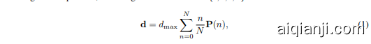
where $d_{\mathrm{max}}$ is a scalar that limits the maximum distance from the anchor center, and ${\mathbf P}(n)$ denotes the probability of each candidate distance of four edges. While GFocal introduces a step forward in handling ambiguity and uncertainty through probability distributions, specific challenges in its regression approach persist: (1) Anchor Dependency: Regression is tied to the anchor box center, limiting prediction diversity and compatibility with anchor-free frameworks. (2) No Iterative Refinement: Predictions are made in one shot without iterative refinements, reducing regression robustness.
其中 $d_{\mathrm{max}}$ 是一个标量,用于限制与锚点中心的最大距离,${\mathbf P}(n)$ 表示四条边每个候选距离的概率。尽管 GFocal 通过概率分布在处理模糊性和不确定性方面迈出了一步,但其回归方法仍存在一些特定挑战:(1) 锚点依赖性:回归与锚点框中心绑定,限制了预测的多样性以及与无锚点框架的兼容性。(2) 无迭代优化:预测是一次性完成的,没有迭代优化,降低了回归的鲁棒性。
(3) Coarse Localization: Fixed distance ranges and uniform bin intervals can lead to coarse localization, especially for small objects, because each bin represents a wide range of possible values.
(3) 粗定位:固定的距离范围和均匀的区间间隔可能导致粗定位,尤其是对于小物体,因为每个区间代表了一个广泛的可能值范围。
Localization Distillation (LD) is a promising approach, demonstrating that transferring localization knowledge is more effective for detection tasks (Zheng et al., 2022). Built upon GFocal, it enhances student models by distilling valuable localization knowledge from teacher models, rather than simply mimicking classification logits or feature maps. Despite its advantages, the method still relies on anchor-based architectures and incurs additional training costs.
定位蒸馏 (Localization Distillation, LD) 是一种有前景的方法,研究表明,在检测任务中传递定位知识更为有效 (Zheng et al., 2022)。该方法基于 GFocal,通过从教师模型中蒸馏出有价值的定位知识来增强学生模型,而不是简单地模仿分类 logits 或特征图。尽管有其优势,但该方法仍然依赖于基于锚点的架构,并会产生额外的训练成本。
4 METHOD
4 方法
We propose D-FINE, a powerful real-time object detector that excels in speed, size, computational cost, and accuracy. D-FINE addresses the shortcomings of existing bounding box regression approaches by leveraging two key components: Fine-grained Distribution Refinement (FDR) and Global Optimal Localization Self-Distillation (GO-LSD), which work in tandem to significantly enhance performance with negligible additional parameters and training time cost.
我们提出了 D-FINE,一种在速度、大小、计算成本和准确性方面表现出色的实时目标检测器。D-FINE 通过利用两个关键组件来解决现有边界框回归方法的不足:细粒度分布优化 (Fine-grained Distribution Refinement, FDR) 和全局最优定位自蒸馏 (Global Optimal Localization Self-Distillation, GO-LSD),这两个组件协同工作,显著提升了性能,同时增加的参数和训练时间成本几乎可以忽略不计。
(1) FDR iterative ly optimizes probability distributions that act as corrections to the bounding box predictions, providing a more fine-grained intermediate representation. This approach captures and optimizes the uncertainty of each edge independently. By leveraging the non-uniform weighting function, FDR allows for more precise and incremental adjustments at each decoder layer, improving localization accuracy and reducing prediction errors. FDR operates within an anchor-free, end-toend framework, enabling a more flexible and robust optimization process.
(1) FDR 通过迭代优化概率分布,作为边界框预测的修正,提供更细粒度的中间表示。该方法独立捕获并优化每条边缘的不确定性。通过利用非均匀权重函数,FDR 允许在每个解码器层进行更精确和逐步的调整,从而提高定位精度并减少预测误差。FDR 在无锚框、端到端的框架内运行,实现了更灵活和鲁棒的优化过程。
(2) GO-LSD distill localization knowledge from refined distributions into shallower layers. As training progresses, the final layer produces increasingly precise soft labels. Shallower layers align their predictions with these labels through GO-LSD, leading to more accurate predictions. As earlystage predictions improve, the subsequent layers can focus on refining smaller residuals. This mutual reinforcement creates a synergistic effect, leading to progressively more accurate localization.
(2) GO-LSD 将定位知识从精炼的分布中蒸馏到较浅的层中。随着训练的进行,最终层产生越来越精确的软标签。较浅的层通过 GO-LSD 将其预测与这些标签对齐,从而产生更准确的预测。随着早期预测的改进,后续层可以专注于精炼较小的残差。这种相互强化产生了协同效应,从而逐步提高定位的准确性。
To further enhance the efficiency of D-FINE, we streamline computationally intensive modules and operations in existing real-time DETR architectures (Zhao et al., 2024), making D-FINE faster and more lightweight. Although these modifications typically result in some performance loss, FDR and GO-LSD effectively mitigate this degradation. The detailed modifications are listed in Table 3.
为进一步提升 D-FINE 的效率,我们简化了现有实时 DETR 架构 (Zhao et al., 2024) 中计算密集型的模块和操作,使 D-FINE 更快、更轻量。尽管这些修改通常会导致一些性能损失,但 FDR 和 GO-LSD 有效地缓解了这种退化。详细修改列于表 3。
4.1 FINE-GRAINED DISTRIBUTION REFINEMENT
4.1 细粒度分布优化
Fine-grained Distribution Refinement (FDR) iterative ly optimizes a fine-grained distribution generated by the decoder layers, as shown in Figure 2. Initially, the first decoder layer predicts preliminary bounding boxes and preliminary probability distributions through a traditional bounding box regression head and a D-FINE head (Both heads are MLP, only the output dimensions are different). Each bounding box is associated with four distributions, one for each edge. The initial bounding boxes serve as reference boxes, while subsequent layers focus on refining them by adjusting distributions in a residual manner. The refined distributions are then applied to adjust the four edges of the corresponding initial bounding box, progressively improving its accuracy with each iteration.
细粒度分布优化 (Fine-grained Distribution Refinement, FDR) 迭代优化由解码器层生成的细粒度分布,如图 2 所示。最初,第一个解码器层通过传统的边界框回归头和一个 D-FINE 头(两者都是 MLP,仅输出维度不同)预测初步的边界框和初步的概率分布。每个边界框与四个分布相关联,每个边对应一个。初始边界框作为参考框,而后续层则通过残差方式调整分布来优化它们。优化后的分布随后用于调整相应初始边界框的四个边,逐步提高其准确性。
Mathematically, let $\mathbf{b}^{0},=,{x,y,W,H}$ denote the initial bounding box prediction, where ${x,y}$ represents the predicted center of the bounding box, and ${W,H}$ represent the width and height of the box. We can then convert ${\bf{b}}^{0}$ into the center coordinates $\mathbf{c}^{\bar{0}}={x,y}$ and the edge distances ${\bf d}^{0},=,{t,b,l,r}$ , which represent the distances from the center to the top, bottom, left, and right edges. For the $l$ -th layer, the refined edge distances $\mathbf{d}^{l}={t^{l},b^{l},l^{l},r^{l}}$ are computed as:
数学上,令 $\mathbf{b}^{0},=,{x,y,W,H}$ 表示初始的边界框预测,其中 ${x,y}$ 表示边界框的预测中心,${W,H}$ 表示边界框的宽度和高度。然后我们可以将 ${\bf{b}}^{0}$ 转换为中心坐标 $\mathbf{c}^{\bar{0}}={x,y}$ 和边缘距离 ${\bf d}^{0},=,{t,b,l,r}$,这些距离表示从中心到上、下、左、右边缘的距离。对于第 $l$ 层,精炼后的边缘距离 $\mathbf{d}^{l}={t^{l},b^{l},l^{l},r^{l}}$ 计算如下:

where $\mathbf P\mathbf r^{l}(n),=,{\mathrm{Pr}{t}^{l}(n),\mathrm{Pr}{b}^{l}(n),\mathrm{Pr}{l}^{l}(n),\mathrm{Pr}{r}^{l}(n)}$ represents four separate distributions, one for each edge. Each distribution predicts the likelihood of candidate offset values for the corresponding edge. These candidates are determined by the weighting function $W(n)$ , where $n$ indexes the discrete bins out of $N$ , with each bin corresponding to a potential edge offset. The weighted sum of the distributions produces the edge offsets. These edge offsets are then scaled by the height $H$ and width $W$ of the initial bounding box, ensuring the adjustments are proportional to the box size.
其中 $\mathbf P\mathbf r^{l}(n),=,{\mathrm{Pr}{t}^{l}(n),\mathrm{Pr}{b}^{l}(n),\mathrm{Pr}{l}^{l}(n),\mathrm{Pr}{r}^{l}(n)}$ 表示四个独立的分布,每个分布对应一条边。每个分布预测对应边的候选偏移值的可能性。这些候选值由加权函数 $W(n)$ 确定,其中 $n$ 索引 $N$ 个离散的区间,每个区间对应一个潜在的边偏移。分布的加权和产生边偏移。然后,这些边偏移通过初始边界框的高度 $H$ 和宽度 $W$ 进行缩放,确保调整与框的大小成比例。

Figure 2: Overview of D-FINE with FDR. The probability distributions that act as a more finegrained intermediate representation are iterative ly refined by the decoder layers in a residual manner. Non-uniform weighting functions are applied to allow for finer localization.
图 2: 带有 FDR 的 D-FINE 概述。作为更细粒度中间表示的概率分布通过解码器层以残差方式迭代优化。应用非均匀加权函数以实现更精细的定位。
The refined distributions are updated using residual adjustments, defined as follows:
使用残差调整更新精炼分布,定义如下:

where logits from the previous layer $l o g i t s^{l-1}(n)$ reflect the confidence in each bin’s offset value for the four edges. The current layer predicts the residual logits $\Delta l o g i t s^{l}(n)$ , which are added to the previous logits to form updated logits $l o g i t s^{l}(n)$ . These updated logits are then normalized using the softmax function, producing the refined probability distributions.
其中前一层的 logits $logits^{l-1}(n)$ 反映了四个边缘每个 bin 偏移值的置信度。当前层预测残差 logits $\Delta logits^{l}(n)$ ,这些残差 logits 被加到前一层的 logits 上,形成更新的 logits $logits^{l}(n)$ 。然后使用 softmax 函数对这些更新的 logits 进行归一化,生成精炼的概率分布。
To facilitate precise and flexible adjustments, the weighting function $W(n)$ is defined as:
为了便于精确和灵活调整,权重函数 $W(n)$ 定义为:

where $a$ and $c$ are hyper-parameters controlling the upper bounds and curvature of the function. As shown in Figure 2, the shape of $W(n)$ ensures that when bounding box prediction is near accurate, small curvature in $W(n)$ allows for finer adjustments. Conversely, if the bounding box prediction is far from accurate, the larger curvature near the edges and the sharp changes at the boundaries of $W(n)$ ensure sufficient flexibility for substantial corrections.
其中 $a$ 和 $c$ 是控制函数上限和曲率的超参数。如图 2 所示,$W(n)$ 的形状确保了当边界框预测接近准确时,$W(n)$ 中的小曲率允许进行更精细的调整。相反,如果边界框预测不准确,$W(n)$ 边缘附近的较大曲率和边界处的急剧变化确保了足够的灵活性以进行大幅修正。
To further improve the accuracy of our distribution predictions and align them with ground truth values, inspired by Distribution Focal Loss (DFL) (Li et al., 2020), we propose a new loss function, Fine-Grained Localization (FGL) Loss, which is computed as:
为了进一步提高我们的分布预测准确性并与真实值对齐,受分布焦点损失 (Distribution Focal Loss, DFL) (Li et al., 2020) 的启发,我们提出了一种新的损失函数,称为细粒度定位 (Fine-Grained Localization, FGL) 损失,其计算公式为:

where $\mathbf{Pr}^{l}(n){k}$ represents the probability distributions corresponding to the $k$ -th prediction. $\phi$ is the relative offset calculated as $\phi\bar{=},({\bf d}^{G T},{-},{\bf\dot{d}}^{0})/{H,H,W,W}$ . $\mathbf{H}^{G T}$ represents the ground truth edgedistance and $n{\leftarrow},n_{\rightarrow}$ are the bin indices adjacent to $\phi$ . The cross-entropy (CE) losses with weights $\omega_{\leftarrow}$ and $\omega_{\rightarrow}$ ensure that the interpolation between bins aligns precisely with the ground truth offset. By incorporating IoU-based weighting, FGL loss encourages distributions with lower uncertainty to become more concentrated, resulting in more precise and reliable bounding box regression.
其中 $\mathbf{Pr}^{l}(n){k}$ 表示第 $k$ 个预测对应的概率分布。$\phi$ 是相对偏移量,计算公式为 $\phi\bar{=},({\bf d}^{G T},{-},{\bf\dot{d}}^{0})/{H,H,W,W}$。$\mathbf{H}^{G T}$ 表示真实边缘距离,$n{\leftarrow},n_{\rightarrow}$ 是与 $\phi$ 相邻的区间索引。带有权重 $\omega_{\leftarrow}$ 和 $\omega_{\rightarrow}$ 的交叉熵 (Cross-Entropy, CE) 损失确保区间之间的插值精确对齐真实偏移量。通过引入基于 IoU 的加权,FGL 损失鼓励不确定性较低的分布更加集中,从而实现更精确和可靠的边界框回归。

Figure 3: Overview of GO-LSD process. Localization knowledge from the final layer’s refined distributions is distilled into shallower layers through DDF loss with decoupled weighting strategies.
图 3: GO-LSD 流程概述。通过解耦加权策略的 DDF 损失,将最终层精炼分布中的定位知识蒸馏到较浅层中。
4.2 GLOBAL OPTIMAL LOCALIZATION SELF-DISTILLATION
4.2 全局最优定位自蒸馏
Global Optimal Localization Self-Distillation (GO-LSD) utilizes the final layer’s refined distribution predictions to distill localization knowledge into the shallower layers, as shown in Figure 3. This process begins by applying Hungarian Matching (Carion et al., 2020) to the predictions from each layer, identifying the local bounding box matches at every stage of the model. To perform a global optimization, GO-LSD aggregates the matching indices from all layers into a unified union set. This union set combines the most accurate candidate predictions across layers, ensuring that they all benefit from the distillation process. In addition to refining the global matches, GO-LSD also optimizes unmatched predictions during training to improve overall stability, leading to improved overall performance. Although the localization is optimized through this union set, the classification task still follows a one-to-one matching principle, ensuring that there are no redundant boxes. This strict matching means that some predictions in the union set are well-localized but have low confidence scores. These low-confidence predictions often represent candidates with precise localization, which still need to be distilled effectively.
全局最优定位自蒸馏 (GO-LSD) 利用最终层的精细化分布预测将定位知识蒸馏到较浅层,如图 3 所示。该过程首先将匈牙利匹配 (Carion et al., 2020) 应用于每一层的预测,以在模型的每个阶段识别局部边界框匹配。为了进行全局优化,GO-LSD 将所有层的匹配索引聚合到一个统一的联合集合中。该联合集合结合了跨层中最准确的候选预测,确保它们都能从蒸馏过程中受益。除了优化全局匹配外,GO-LSD 还在训练过程中优化未匹配的预测,以提高整体稳定性,从而提升整体性能。尽管定位通过该联合集合进行了优化,但分类任务仍遵循一对一匹配原则,确保没有冗余框。这种严格的匹配意味着联合集合中的一些预测定位良好但置信度较低。这些低置信度预测通常代表具有精确定位的候选框,仍然需要有效地蒸馏。
To address this, we introduce Decoupled Distillation Focal (DDF) Loss, which applies decoupled weighting strategies to ensure that high-IoU but low-confidence predictions are given appropriate weight. The DDF Loss also weights matched and unmatched predictions according to their quantity, balancing their overall contribution and individual losses. This approach results in more stable and effective distillation. The Decoupled Distillation Focal Loss $\mathcal{L}_{\mathrm{DDF}}$ is then formulated as:
为了解决这个问题,我们引入了解耦蒸馏焦点 (Decoupled Distillation Focal, DDF) 损失函数,它采用了解耦加权策略,以确保高 IoU 但低置信度的预测被赋予适当的权重。DDF 损失还根据匹配和不匹配预测的数量进行加权,平衡它们的整体贡献和个体损失。这种方法使得蒸馏过程更加稳定和有效。解耦蒸馏焦点损失 $\mathcal{L}_{\mathrm{DDF}}$ 的公式如下:
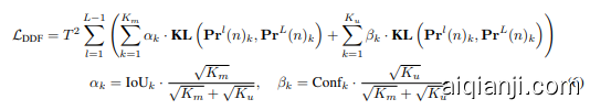
where $\mathbf{KL}$ represents the Kullback-Leibler divergence (Hinton et al., 2015), and $T$ is the temperature parameter used for smoothing logits. The distillation loss for the $k$ -th matched prediction is weighted by $\alpha_{k}$ , where $K_{m}$ and $K_{u}$ are the numbers of matched and unmatched predictions, respectively. For the $k$ -th unmatched prediction, the weight is $\beta_{k}$ , with $\mathrm{Conf}_{k}$ denoting the classification confidence.
其中 $\mathbf{KL}$ 表示 Kullback-Leibler 散度 (Hinton et al., 2015),$T$ 是用于平滑 logits 的温度参数。第 $k$ 个匹配预测的蒸馏损失由 $\alpha_{k}$ 加权,其中 $K_{m}$ 和 $K_{u}$ 分别是匹配和不匹配预测的数量。对于第 $k$ 个不匹配预测,权重为 $\beta_{k}$,$\mathrm{Conf}_{k}$ 表示分类置信度。
5 EXPERIMENTS
5 实验
5.1 EXPERIMENT SETUP
5.1 实验设置
To validate the effectiveness of our proposed methods, we conduct experiments on the COCO (Lin et al., 2014a) and Objects365 (Shao et al., 2019) datasets. We evaluate our D-FINE using the standard COCO metrics, including Average Precision (AP) averaged over IoU thresholds from 0.50 to 0.95, as well as AP at specific thresholds $\mathrm{\DeltaAP_{50}}$ and $\mathrm{AP_{75}}$ ) and AP across different object scales: small $(\mathrm{AP}{S})$ , medium $(\mathbf{AP}{M})$ , and large $(\mathbf{A}\mathbf{P}_{L})$ . Additionally, we provide model efficiency metrics by reporting the number of parameters (#Params.), computational cost (GFLOPs), and end-to-end latency. The latency is measured using TensorRT FP16 on an NVIDIA T4 GPU.
为了验证我们提出方法的有效性,我们在 COCO (Lin et al., 2014a) 和 Objects365 (Shao et al., 2019) 数据集上进行了实验。我们使用标准的 COCO 指标评估了我们的 D-FINE,包括在 IoU 阈值从 0.50 到 0.95 之间平均的平均精度 (AP),以及特定阈值 ($\mathrm{\DeltaAP_{50}}$ 和 $\mathrm{AP_{75}}$) 下的 AP,以及不同物体尺度下的 AP:小 ($\mathrm{AP}{S}$)、中 ($\mathbf{AP}{M}$) 和大 ($\mathbf{A}\mathbf{P}_{L}$)。此外,我们还通过报告参数量 (#Params.)、计算成本 (GFLOPs) 和端到端延迟来提供模型效率指标。延迟是在 NVIDIA T4 GPU 上使用 TensorRT FP16 测量的。
Table 1: Performance comparison of various real-time object detectors on COCO val2017.
$\star$ : NMS is tuned with a confidence threshold of 0.01.
5.2 COMPARISON WITH REAL-TIME DETECTORS
5.2 与实时检测器的比较
Table 1 provides a comprehensive comparison between D-FINE and various real-time object detectors on COCO val2017. D-FINE achieves an excellent balance between efficiency and accuracy across multiple metrics. Specifically, D-FINE-L attains an AP of $54.0%$ with 31M parameters and 91 GFLOPs, maintaining a low latency of $8.07~\mathrm{ms}$ . Additionally, D-FINE $\mathbf{\deltaX}$ achieves an AP of $55.8%$ with 62M parameters and 202 GFLOPs, operating with a latency of $12.89,\mathrm{ms}$ .
表 1: 提供了 D-FINE 与各种实时目标检测器在 COCO val2017 上的全面比较。D-FINE 在多个指标上实现了效率与准确性的优秀平衡。具体而言,D-FINE-L 在 31M 参数和 91 GFLOPs 的情况下达到了 $54.0%$ 的 AP,同时保持了 $8.07~\mathrm{ms}$ 的低延迟。此外,D-FINE $\mathbf{\deltaX}$ 在 62M 参数和 202 GFLOPs 的情况下达到了 $55.8%$ 的 AP,运行延迟为 $12.89,\mathrm{ms}$。
As depicted in Figure 1, which shows scatter plots of latency vs. AP, parameter count vs. AP, and FLOPs vs. AP, D-FINE consistently outperforms other state-of-the-art models across all key dimensions. D-FINE-L achieves a higher AP $(54.0%)$ compared to YOLOv10-L $(53.2%)$ , RTDETR-R50 $(53.1%)$ , and LW-DETR-X $(53.0%)$ , while requiring fewer computational resources (91 GFLOPs vs. 120, 136, and 174). Similarly, D-FINE $\mathbf{\deltaX}$ surpasses YOLOv10-X and RT-DETR-R101 by achieving superior performance $55.8%$ AP vs. $54.4%$ and $54.3%$ ) and demonstrating greater efficiency in terms of lower parameter count, GFLOPs, and latency.
如图 1 所示,图中展示了延迟与 AP、参数量与 AP 以及 FLOPs 与 AP 的散点图,D-FINE 在所有关键维度上始终优于其他最先进的模型。D-FINE-L 实现了更高的 AP $(54.0%)$,而 YOLOv10-L $(53.2%)$、RTDETR-R50 $(53.1%)$ 和 LW-DETR-X $(53.0%)$ 则需要更多的计算资源(91 GFLOPs 对比 120、136 和 174)。同样,D-FINE $\mathbf{\deltaX}$ 超越了 YOLOv10-X 和 RT-DETR-R101,实现了更高的性能 $(55.8% AP 对比 54.4% 和 54.3%)$,并在更低的参数量、GFLOPs 和延迟方面表现出更高的效率。
We further pretrain D-FINE and YOLOv10 on the Objects365 dataset (Shao et al., 2019), before finetuning them on COCO. After pre training, both D-FINE-L and D-FINE $\mathbf{\deltaX}$ exhibit significant performance improvements, achieving AP of $57.1%$ and $59.3%$ , respectively. These enhancements enable them to outperform YOLOv10-L and YOLOv10-X by $3.1%$ and $4.4%$ AP, thereby positioning them as the top-performing models in this comparison. What’s more, following the pre training protocol of YOLOv8 (Glenn., 2023), YOLOv10 is pretrained on Objects365 for 300 epochs. In contrast, D-FINE requires only 21 epochs to achieve its substantial performance gains. These findings corroborate the conclusions of LW-DETR (Chen et al., 2024), demonstrating that DETR-based models benefit substantially more from pre training compared to other detectors like YOLOs.
我们进一步在Objects365数据集 (Shao et al., 2019) 上对D-FINE和YOLOv10进行预训练,随后在COCO上进行微调。预训练后,D-FINE-L和D-FINE $\mathbf{\deltaX}$ 均表现出显著的性能提升,分别达到了 $57.1%$ 和 $59.3%$ 的AP值。这些改进使它们在AP上分别超越了YOLOv10-L和YOLOv10-X $3.1%$ 和 $4.4%$ ,从而在本次对比中成为表现最佳的模型。此外,按照YOLOv8 (Glenn., 2023) 的预训练协议,YOLOv10在Objects365上预训练了300个epoch。相比之下,D-FINE仅需21个epoch即可实现其显著的性能提升。这些发现验证了LW-DETR (Chen et al., 2024) 的结论,表明基于DETR的模型相比YOLO等其他检测器从预训练中获益更多。
Table 2: Effectiveness of FDR and GO-LSD across various DETR models on COCO val2017.
表 2: FDR 和 GO-LSD 在各种 DETR 模型上在 COCO val2017 上的效果。
| 模型 | #参数 | #训练轮数 | Apval | APg | AP"g | APyal | AP%al | APyal |
|---|---|---|---|---|---|---|---|---|
| Deformable-DETR | 40M | 12 | 43.7 | 62.2 | 46.9 | 26.4 | 46.4 | 57.9 |
| + FDR & GO-LSD | 40M | 12 | 47.1 (+3.4) | 64.7 | 50.8 | 29.0 | 50.3 | 62.8 |
| DAB-DETR | 48M | 12 | 44.2 | 62.5 | 47.3 | 27.5 | 47.1 | 58.6 |
| + FDR & GO-LSD | 48M | 12 | 49.5 (+5.3) | 67.2 | 54.1 | 31.8 | 53.2 | 63.3 |
| DN-DETR | 48M | 12 | 46.0 | 64.8 | 49.9 | 27.7 | 49.1 | 62.3 |
| + FDR & GO-LSD | 48M | 12 | 49.7 (+3.7) | 67.5 | 54.4 | 31.8 | 53.4 | 63.8 |
| DINO | 47M | 12 | 49.0 | 66.6 | 53.5 | 32.0 | 52.3 | 63.0 |
| + FDR & GO-LSD | 47M | 12 | 51.6 (+2.6) | 68.6 | 56.3 | 33.8 | 55.6 | 65.3 |
| DINO | 47M | 24 | 50.4 | 68.3 | 54.8 | 33.3 | 53.7 | 64.8 |
| + FDR & GO-LSD | 47M | 24 | 52.4 (+2.0) | 69.5 | 56.9 | 34.6 | 55.7 | 66.2 |
5.3 EFFECTIVENESS ON VARIOUS DETR MODELS
5.3 各种 DETR 模型的有效性
Table 2 demonstrates the effectiveness of our proposed FDR and GO-LSD methods across multiple DETR-based object detectors on COCO val2017. Our methods are designed for flexibility and can be seamlessly integrated into any DETR architecture, significantly enhancing performance without increasing the number of parameters and computational burden. Incorporating FDR and GO-LSD into Deformable DETR, DAD-DETR, DN-DETR, and DINO consistently improves detection accuracy, with gains ranging from $2.0%$ to $5.3%$ . These results highlight the effectiveness of FDR and GO-LSD in enhancing localization precision and maximizing efficiency, demonstrating their adaptability and substantial impact across various end-to-end detection frameworks.
表 2 展示了我们提出的 FDR 和 GO-LSD 方法在 COCO val2017 数据集上对多种基于 DETR 的目标检测器的有效性。我们的方法设计灵活,可以无缝集成到任何 DETR 架构中,在不增加参数数量和计算负担的情况下显著提升性能。将 FDR 和 GO-LSD 集成到 Deformable DETR、DAD-DETR、DN-DETR 和 DINO 中,检测精度一致提高,提升范围从 $2.0%$ 到 $5.3%$ 不等。这些结果突显了 FDR 和 GO-LSD 在提升定位精度和最大化效率方面的有效性,展示了它们在各种端到端检测框架中的适应性和显著影响。
5.4 ABLATION STUDY
5.4 消融研究
5.4.1 THE ROADMAP TO D-FINE
5.4.1 D-FINE 的路线图
Table 3 showcases the stepwise progression from the baseline model (RT-DETR-HGNetv2-L (Zhao et al., 2024)) to our proposed D-FINE framework. Starting with the baseline metrics of $53.0%$ AP, 32M parameters, 110 GFLOPs, and $9.25~\mathrm{ms}$ latency, we first remove all the decoder projection layers. This modification reduces GFLOPs to 97 and cuts the latency to $8.02~\mathrm{ms}$ , although it decreases AP to $52.4%$ . To address this drop, we introduce the Target Gating Layer, which recovers the AP to $52.8%$ with only a marginal increase in computational cost.
表 3 展示了从基线模型 (RT-DETR-HGNetv2-L (Zhao et al., 2024)) 到我们提出的 D-FINE 框架的逐步进展。从基线指标 53.0% AP、32M 参数、110 GFLOPs 和 9.25 ms 延迟开始,我们首先移除了所有的解码器投影层。这一修改将 GFLOPs 减少到 97,并将延迟降低到 8.02 ms,尽管它将 AP 降低到 52.4%。为了解决这一下降,我们引入了目标门控层 (Target Gating Layer),将 AP 恢复到 52.8%,而计算成本仅略有增加。
The Target Gating Layer is strategically placed after the decoder’s cross-attention module, replacing the residual connection. It allows queries to dynamically switch their focus on different targets across layers, effectively preventing information entanglement. The mechanism operates as follows:
目标门控层策略性地放置在解码器的交叉注意力模块之后,替代了残差连接。它允许查询在不同层之间动态切换对不同目标的关注,有效防止信息纠缠。该机制的工作原理如下:

where $\mathbf{x_{1}}$ represents the previous queries and $\mathbf{x_{2}}$ is the cross-attention result. $\sigma$ is the sigmoid activation function applied to the concatenated outputs, and $[.]$ represents the concatenation operation.
其中,$\mathbf{x_{1}}$ 代表先前的查询,$\mathbf{x_{2}}$ 是交叉注意力的结果。$\sigma$ 是应用于拼接输出的 sigmoid 激活函数,$[.]$ 表示拼接操作。
Next, we replace the encoder’s CSP layers with GELAN layers (Wang & Liao, 2024). This substitution increases AP to $53.5%$ but also raises the parameter count, GFLOPs, and latency. To mitigate the increased complexity, we reduce the hidden dimension of GELAN, which balances the model’s
接下来,我们将编码器的 CSP 层替换为 GELAN 层 (Wang & Liao, 2024)。这一替换将 AP 提高到 $53.5%$,但也增加了参数数量、GFLOPs 和延迟。为了缓解复杂度的增加,我们减少了 GELAN 的隐藏维度,从而平衡了模型。
Table 3: Step-by-step modifications from baseline model to D-FINE. Each step shows changes in AP, the number of parameters, latency, and FLOPs.
表 3: 从基线模型到 D-FINE 的逐步修改。每一步都展示了 AP、参数量、延迟和 FLOPs 的变化。
| 模型 | APual | #Params. | Latency(ms) | GFLOPs |
|---|---|---|---|---|
| 基线: RT-DETR-HGNetv2-L (Zhao et al., 2024) | 53.0 | 32M | 9.25 | 110 |
| 移除解码器投影层 | 52.4 | 32M | 8.02 | 97 |
| + 目标门控层 | 52.8 | 33M | 8.15 | 98 |
| 编码器 CSP 层 → GELAN (Wang & Liao, 2024) | 53.5 | 46M | 10.69 | 167 |
| 将 GELAN 的隐藏维度减半 | 52.8 | 31M | 8.01 | 91 |
| 非均匀采样点 (S: 3, M: 6, L: 3) | 52.9 | 31M | 7.90 | 91 |
| RT-DETRv2 训练策略 (Lv et al., 2024) | 53.0 | 31M | 7.90 | 91 |
| +FDR | 53.5 | 31M | 8.07 | 91 |
| +GO-LSD | 54.0 (+1.0) 31M (-3%) | 8.07(-13%) | 91 (-17%) |
Table 4: Hyper parameter ablation studies on D-FINE-L. $\epsilon$ is a very small value. $\widetilde{a}_{\cdot}$ ,c indicate that $a$ and $c$ are learnable para m e t ers.
表 4: D-FINE-L 的超参数消融研究。$\epsilon$ 是一个非常小的值。$\widetilde{a}_{\cdot}$,c 表示 $a$ 和 $c$ 是可学习的参数。
| a,c | ||||
|---|---|---|---|---|
| APval | 52.75 | 53.053.3 | 53.2 53.2 53.1 | |
| N | 4 | 8 | 16 32 | 64 128 |
| APval | 53.353.453.553.7 53.653.6 | |||
| T | 1 | 2.5 5 | 7.5 | 10 20 |
| APval | 53.253.75 | 54.053.853.753.5 |
Table 5: Distillation methods comparison in terms of performance, training time, and GPU memory usage. GO-LSD achieves the highest $\boldsymbol{\mathrm{AP}}^{v a l}$ with minimal additional training cost.
表 5: 蒸馏方法在性能、训练时间和 GPU 内存使用方面的比较。GO-LSD 以最小的额外训练成本实现了最高的 $\boldsymbol{\mathrm{AP}}^{v a l}$。
| 方法 | APval | 时间/轮次 | 内存 |
|---|---|---|---|
| baseline | 53.0 | 29分钟 | 8552M |
| Logit Mimicking | 52.6 | 31分钟 | 8554M |
| FeatureImitation | 52.9 | 31分钟 | 8554M |
| baseline+FDR | 53.8 | 30分钟 | 8730M |
| LocalizationDistill | 53.7 | 31分钟 | 8734M |
| GO-LSD | 54.5 | 31分钟 | 8734M |
complexity and maintains AP at $52.8%$ while improving efficiency. We further optimize the sampling points by implementing uneven sampling across different scales (S: 3, M: 6, L: 3), which slightly increases AP to $52.9%$ . However, alternative sampling combinations such as (S: 6, M: 3, L: 3) and $(\mathrm{S};3,\mathrm{M};3,\mathrm{L};6)$ result in a minor performance drop of $0.1%$ AP. Adopting the RT-DETRv2 training strategy (Lv et al., 2024) (see Appendix A.1.1 for details) enhances AP to $53.0%$ without affecting the number of parameters or latency. Finally, the integration of FDR and GO-LSD modules elevates AP to $54.0%$ , achieving a $13%$ reduction in latency and a $17%$ reduction in GFLOPs compared to the baseline model. These incremental modifications demonstrate the robustness and effectiveness of our D-FINE framework.
复杂性并保持 AP 在 $52.8%$,同时提高效率。我们通过在不同尺度上实施不均匀采样(S: 3, M: 6, L: 3)进一步优化采样点,将 AP 略微提升至 $52.9%$。然而,其他采样组合如(S: 6, M: 3, L: 3)和 $(\mathrm{S};3,\mathrm{M};3,\mathrm{L};6)$ 导致 AP 性能略微下降 $0.1%$。采用 RT-DETRv2 训练策略(Lv 等,2024)(详见附录 A.1.1)将 AP 提升至 $53.0%$,而不影响参数数量或延迟。最后,FDR 和 GO-LSD 模块的集成将 AP 提升至 $54.0%$,与基线模型相比,延迟减少 $13%$,GFLOPs 减少 $17%$。这些渐进式修改展示了我们 D-FINE 框架的稳健性和有效性。
5.4.2 HYPER PARAMETER SENSITIVITY ANALYSIS
5.4.2 超参数敏感性分析
Section 5.4.1 presents a subset of hyper parameter ablation studies evaluating the sensitivity of our model to key parameters in the FDR and GO-LSD modules. We examine the weighting function parameters $a$ and $c$ , the number of distribution bins $N$ , and the temperature $T$ used for smoothing logits in the KL divergence.
第5.4.1节介绍了一部分超参数消融研究,评估了我们的模型对FDR和GO-LSD模块中关键参数的敏感性。我们考察了权重函数参数 $a$ 和 $c$、分布区间数量 $N$ 以及用于平滑KL散度中logits的温度 $T$。
(1) Setting $\begin{array}{r}{a=\frac{1}{2}}\end{array}$ and $c=\textstyle{\frac{1}{4}}$ yields the highest AP of $53.3%$ . Notably, treating $a$ and $c$ as learnable parameters $(\widetilde{\boldsymbol{a}},\widetilde{\boldsymbol{c}})$ slightly decreases AP to $53.1%$ , suggesting that fixed values simplify the optimization process. When $c$ is extremely large, the weighting function approximates the linear function with equal intervals, resulting in a suboptimal AP of $53.0%$ . Additionally, values of $a$ that are too large or too small can reduce fineness or limit flexibility, adversely affecting localization precision. (2) Increasing the number of distribution bins improves performance, with a maximum AP of $53.7%$ achieved at $N=32$ . Beyond $N=32$ , no significant gain is observed. (3) The temperature $T$ controls the smoothing of logits during distillation. An optimal AP of $54.0%$ is achieved at $T,=,5$ , indicating a balance between softening the distribution and preserving effective knowledge transfer.
(1) 设置 $\begin{array}{r}{a=\frac{1}{2}}\end{array}$ 和 $c=\textstyle{\frac{1}{4}}$ 时,AP 达到最高的 $53.3%$。值得注意的是,将 $a$ 和 $c$ 作为可学习参数 $(\widetilde{\boldsymbol{a}},\widetilde{\boldsymbol{c}})$ 时,AP 略微下降至 $53.1%$,这表明固定值简化了优化过程。当 $c$ 非常大时,加权函数近似于等间隔的线性函数,导致 AP 降至 $53.0%$。此外,$a$ 值过大或过小都会降低精细度或限制灵活性,从而对定位精度产生不利影响。(2) 增加分布区间的数量可以提高性能,在 $N=32$ 时达到最大 AP 值 $53.7%$。超过 $N=32$ 后,未观察到显著增益。(3) 温度 $T$ 控制蒸馏过程中 logits 的平滑度。在 $T,=,5$ 时达到最佳 AP 值 $54.0%$,表明在软化分布和保持有效知识传递之间取得了平衡。

Figure 4: Visualization of FDR across detection scenarios with initial and refined bounding boxes, along with unweighted and weighted distributions, highlighting improved localization accuracy.
图 4: 在不同检测场景下,使用初始和优化后的边界框以及未加权和加权分布的 FDR 可视化,展示了定位精度的提升。
5.4.3 COMPARISON OF DISTILLATION METHODS
5.4.3 蒸馏方法比较
Section 5.4.1 compares different distillation methods based on performance, training time, and GPU memory usage. The baseline model achieves an AP of $53.0%$ , with a training time of 29 minutes per epoch and memory usage of $8552,\mathrm{MB}$ on four NVIDIA RTX 4090 GPUs. Due to the instability of one-to-one matching in DETR, traditional distillation techniques like Logit Mimicking and Feature Imitation do not improve performance; Logit Mimicking reduces AP to $52.6%$ , while Feature Imitation achieves $52.9%$ . Incorporating our FDR module increases AP to $53.8%$ with minimal additional training cost. Applying vanilla Localization Distillation (Zheng et al., 2022) further increases AP to $53.7%$ . Our GO-LSD method achieves the highest AP of $54.5%$ , with only a $6%$ increase in training time and a $2%$ rise in memory usage compared to the baseline. Notably, no lightweight optimization s are applied in this comparison, focusing purely on distillation performance.
第5.4.1节基于性能、训练时间和GPU内存使用情况比较了不同的蒸馏方法。基线模型在四个NVIDIA RTX 4090 GPU上实现了$53.0%$的AP(平均精度),每个epoch的训练时间为29分钟,内存使用量为$8552,\mathrm{MB}$。由于DETR中一对一匹配的不稳定性,传统的蒸馏技术如Logit Mimicking和Feature Imitation并未提升性能;Logit Mimicking将AP降低至$52.6%$,而Feature Imitation达到了$52.9%$。引入我们的FDR模块后,AP提升至$53.8%$,且额外训练成本最小。应用原始的Localization Distillation (Zheng et al., 2022)进一步将AP提升至$53.7%$。我们的GO-LSD方法实现了最高的$54.5%$的AP,与基线相比,训练时间仅增加了$6%$,内存使用量增加了$2%$。值得注意的是,在此比较中未应用任何轻量化优化,仅关注蒸馏性能。
5.5 VISUALIZATION ANALYSIS
5.5 可视化分析
Figure 4 illustrates the process of FDR across various detection scenarios. We display the filtered detection results with two bounding boxes overlaid on the images. The red boxes represent the initial predictions from the first decoder layer, while the green boxes denote the refined predictions from the final decoder layer. The final predictions align more closely with the target objects. The first row under the images shows the unweighted probability distributions for the four edges (left, top, right, bottom). The second row shows the weighted distributions, where the weighting function $W(n)$ has been applied. The red curves represent the initial distributions, while the green curves show the final, refined distributions. The weighted distributions emphasize finer adjustments near accurate predictions and allow for enabling rapid changes for larger adjustments, further illustrating how FDR refines the offsets of initial bounding boxes, leading to increasingly precise localization.
图 4: 展示了 FDR 在不同检测场景中的过程。我们在图像上叠加了两个边界框来显示过滤后的检测结果。红色框表示来自第一个解码器层的初始预测,绿色框表示来自最终解码器层的优化预测。最终预测与目标对象更加吻合。图像下方的第一行显示了四个边缘(左、上、右、下)的未加权概率分布。第二行显示了加权分布,其中应用了加权函数 $W(n)$。红色曲线表示初始分布,绿色曲线表示最终的优化分布。加权分布强调了在准确预测附近进行更精细的调整,并允许在较大调整时进行快速变化,进一步说明了 FDR 如何优化初始边界框的偏移,从而实现越来越精确的定位。
In this paper, we introduce D-FINE, a powerful real-time object detector that redefines the bounding box regression task in DETR models through Fine-grained Distribution Refinement (FDR) and Global Optimal Localization Self-Distillation (GO-LSD). Experimental results on the COCO dataset demonstrate that D-FINE achieves state-of-the-art accuracy and efficiency, surpassing all existing real-time detectors. Limitation and Future Work: However, the performance gap between lighter D-FINE models and other compact models remains small. One possible reason is that shallow decoder layers may yield less accurate final-layer predictions, limiting the effectiveness of distilling localization knowledge into earlier layers. Addressing this challenge necessitates enhancing the localization capabilities of lighter models without increasing inference latency. Future research could investigate advanced architectural designs or novel training paradigms that allow for the inclusion of additional sophisticated decoder layers during training while maintaining lightweight inference by simply discarding them at test time. We hope D-FINE inspires further advancements in this area.
本文介绍了 D-FINE,这是一种强大的实时目标检测器,通过细粒度分布优化(FDR)和全局最优定位自蒸馏(GO-LSD)重新定义了 DETR 模型中的边界框回归任务。在 COCO 数据集上的实验结果表明,D-FINE 在准确性和效率上达到了最先进的水平,超越了所有现有的实时检测器。局限性与未来工作:然而,较轻的 D-FINE 模型与其他紧凑模型之间的性能差距仍然较小。一个可能的原因是浅层解码器层可能产生不太准确的最终层预测,限制了将定位知识蒸馏到较早层的效果。解决这一挑战需要在增加推理延迟的情况下增强较轻模型的定位能力。未来的研究可以探索先进的架构设计或新颖的训练范式,允许在训练期间包含更多复杂的解码器层,同时在测试时通过简单地丢弃这些层来保持轻量级推理。我们希望 D-FINE 能够激发该领域的进一步进展。
REFERENCES
参考文献
Xizhou Zhu, Weijie Su, Lewei Lu, Bin Li, Xiaogang Wang, and Jifeng Dai. Deformable detr: Deformable transformers for end-to-end object detection. In International Conference on Learning Representations, 2020.
Xizhou Zhu, Weijie Su, Lewei Lu, Bin Li, Xiaogang Wang, and Jifeng Dai. Deformable DETR: 用于端到端目标检测的可变形 Transformer. 在 International Conference on Learning Representations, 2020.
A APPENDIX
A 附录
A.1 IMPLEMENTATION DETAILS
A.1 实现细节
A.1.1 HYPER PARAMETER CONFIGURATIONS
A.1.1 超参数配置
Table 6 summarizes the hyper parameter configurations for the D-FINE models. All variants use HGNetV2 backbones pretrained on ImageNet (Cui et al., 2021; Russ a kov sky et al., 2015) and the AdamW optimizer. D-FINE-X is set with an embedding dimension of 384 and a feed forward dimension of 2048, while the other models use 256 and 1024, respectively. The D-FINE-X and D-FINE-L have 6 decoder layers, while D-FINE-M and D-FINE-S have 4 and 3 decoder layers. The GELAN module progressively reduces hidden dimension and depth from D-FINE-X with 192 dimensions and 3 layers to D-FINE-S with 64 dimensions and 1 layer. The base learning rate and weight decay for D-FINE-X and D-FINE-L are $2.5\times10^{-4}$ and $1.25\times10^{-4}$ , respectively, while D-FINE-M and D-FINE-S use $2\times10^{-4}$ and $1\times10^{-4}$ . Smaller models also have higher backbone learning rates than larger models. The total batch size is 32 across all variants. Training schedules include 72 epochs with advanced augmentation (Random Photometric Distort, Random Zoom Out, Random I oU Crop, and R Multi Scale Input) followed by 2 epochs without advanced augmentation for D-FINE-X and D-FINE-L, and 120 epochs with advanced augmentation followed by 4 epochs without advanced augmentation for D-FINE-M and D-FINE-S (RT-DETRv2 Training Strategy (Lv et al., 2024) in Table 3). The number of pre training epochs is 21 for D-FINE-X and DFINE-L models, while for D-FINE-M and D-FINE-S models, it ranges from 28 to 29 epochs.
表 6 总结了 D-FINE 模型的超参数配置。所有变体都使用在 ImageNet 上预训练的 HGNetV2 骨干网络(Cui 等, 2021; Russakovsky 等, 2015)和 AdamW 优化器。D-FINE-X 的嵌入维度设置为 384,前馈维度为 2048,而其他模型分别使用 256 和 1024。D-FINE-X 和 D-FINE-L 有 6 个解码器层,而 D-FINE-M 和 D-FINE-S 分别有 4 层和 3 层。GELAN 模块从 D-FINE-X 的 192 维度和 3 层逐步减少到 D-FINE-S 的 64 维度和 1 层。D-FINE-X 和 D-FINE-L 的基础学习率和权重衰减分别为 $2.5\times10^{-4}$ 和 $1.25\times10^{-4}$,而 D-FINE-M 和 D-FINE-S 使用 $2\times10^{-4}$ 和 $1\times10^{-4}$。较小的模型也比较大的模型具有更高的骨干网络学习率。所有变体的总批处理大小为 32。训练计划包括 72 个带有高级增强(随机光度失真、随机缩小、随机 IoU 裁剪和随机多尺度输入)的 epoch,随后是 2 个不带高级增强的 epoch(适用于 D-FINE-X 和 D-FINE-L),以及 120 个带有高级增强的 epoch,随后是 4 个不带高级增强的 epoch(适用于 D-FINE-M 和 D-FINE-S)(参见表 3 中的 RT-DETRv2 训练策略(Lv 等, 2024))。D-FINE-X 和 D-FINE-L 模型的预训练 epoch 数为 21,而 D-FINE-M 和 D-FINE-S 模型的预训练 epoch 数在 28 到 29 之间。
Table 6: Hyper parameter configurations for different D-FINE models.
表 6: 不同 D-FINE 模型的超参数配置。
| 设置 | D-FINE-X | D-FINE-L | D-FINE-M | D-FINE-S |
|---|---|---|---|---|
| 主干网络名称 | HGNetv2-B5 | HGNetv2-B4 | HGNetv2-B2 | HGNetv2-B0 |
| 优化器 | AdamW | AdamW | AdamW | AdamW |
| 嵌入维度 | 384 | 256 | 256 | 256 |
| 前馈维度 | 2048 | 1024 | 1024 | 1024 |
| GELAN 隐藏维度 | 192 | 128 | 128 | 64 |
| GELAN 深度 | 3 | 3 | 2 | 1 |
| 解码器层数 | 6 | 6 | 4 | 3 |
| 查询数 | 300 | 300 | 300 | 300 |
| a,cin W(n) | 0.5,0.125 | 0.5,0.25 | 0.5,0.25 | 0.5,0.25 |
| 分箱数 N | 32 | 32 | 32 | 32 |
| 采样点数 | (S:3, M: 6, L: 3) | (S:3,M: 6,L: 3) | (S:3, M: 6,L: 3) | (S:3, M: 6, L: 3) |
| 温度 T | 5 | 5 | 5 | 5 |
| 基础学习率 | 2.5e-4 | 2.5e-4 | 2e-4 | 2e-4 |
| 主干网络学习率 | 2.5e-6 | 1.25e-5 | 2e-5 | 1e-4 |
| 权重衰减 | 1.25e-4 | 1.25e-4 | 1e-4 | 1e-4 |
| LvFL 权重 | 1 | 1 | 1 | 1 |
| LBBox 权重 | 5 | 5 | 5 | 5 |
| LGIOU 权重 | 2 | 2 | 2 | 2 |
| LFGL 权重 | 0.15 | 0.15 | 0.15 | 0.15 |
| LDDF 权重 | 1.5 | 1.5 | 1.5 | 1.5 |
| 总批量大小 | 32 | 32 | 32 | 32 |
| EMA 衰减 | 0.9999 | 0.9999 | 0.9999 | 0.9999 |
| 训练轮数 (带/不带 Adv. Aug.) | 72+2 | 72+2 | 120 + 4 | 120 + 4 |
| 训练轮数 (预训练 + 微调) | 21 + 31 | 21 + 32 | 29 + 49 | 28+58 |
A.1.2 DATASETS SETTINGS
A.1.2 数据集设置
For pre training, following the approach in (Chen et al., 2022b; Zhang et al., 2022; Chen et al., 2024), we combine the images from the Objects365 (Shao et al., 2019) train set with the validate set, excluding the first $5\mathrm{k}$ images. To further improve training efficiency, we resize all images with resolutions exceeding $640\times640$ down to $640\times640$ beforehand. We use the standard COCO2017 (Lin et al., 2014b) data splitting policy, training on COCO train2017, and evaluating on COCO val2017.
在预训练阶段,我们遵循 (Chen et al., 2022b; Zhang et al., 2022; Chen et al., 2024) 的方法,将 Objects365 (Shao et al., 2019) 训练集中的图像与验证集合并,并排除前 $5\mathrm{k}$ 幅图像。为了进一步提高训练效率,我们事先将所有分辨率超过 $640\times640$ 的图像调整为 $640\times640$。我们采用标准的 COCO2017 (Lin et al., 2014b) 数据分割策略,在 COCO train2017 上进行训练,并在 COCO val2017 上进行评估。
Figure 5 demonstrates the robustness of the D-FINE-X model, visualizing its predictions in various challenging scenarios. These include occlusion, low-light conditions, motion blur, depth of field effects, rotation, and densely populated scenes with numerous objects in close proximity. Despite these difficulties, the model accurately identifies and localizes objects, such as animals, vehicles, and people. This visualization highlights the model’s ability to handle complex real-world conditions while maintaining robust detection performance.
图 5 展示了 D-FINE-X 模型的鲁棒性,可视化了其在各种具有挑战性的场景中的预测结果。这些场景包括遮挡、低光条件、运动模糊、景深效果、旋转以及物体密集且距离较近的拥挤场景。尽管面临这些困难,该模型仍能准确识别和定位动物、车辆和人物等对象。这一可视化结果突显了模型在处理复杂现实世界条件的同时,仍能保持稳健的检测性能。

Figure 5: Visualization of D-FINE-X (without pre-training on Objects365) predictions under challenging conditions, including occlusion, low light, motion blur, depth of field effects, rotation, and densely populated scenes (confidence threshold $=!0.5_{\cdot}$ ).
图 5: 在遮挡、低光照、运动模糊、景深效果、旋转和密集场景等挑战性条件下,D-FINE-X (未在 Objects365 上进行预训练) 预测的可视化结果 (置信度阈值 $=!0.5_{\cdot}$)。
Table 7 presents a comprehensive comparison of D-FINE models with various lightweight real-time object detectors in the S and M model sizes on the COCO val2017. D-FINE-S achieves an impressive AP of $48.5%$ , surpassing other lightweight models such as Gold-YOLO-S $(46.4%)$ and RT-DETRv2-S $(48.1%)$ , while maintaining a low latency of $3.49~\mathrm{ms}$ with only 10.2M parameters and 25.2 GFLOPs. Pre training on Objects365 further boosts D-FINE-S to $50.7%$ , marking an improvement of $+2.2%$ . Similarly, D-FINE-M attains an AP of $52.3%$ with 19.2M parameters and 56.6 GFLOPs at $5.62,\mathrm{ms}$ , outperforming YOLOv10-M $(51.1%)$ and RT-DETRv2-M $(49.9%)$ . Pre training on Objects365 consistently enhances D-FINE-M, yielding a $+2.8%$ gain. These results demonstrate that D-FINE models strike an excellent balance between accuracy and efficiency, consistently surpassing other state-of-the-art lightweight detectors while preserving real-time performance.
表 7: 在 COCO val2017 数据集上,D-FINE 模型与 S 和 M 模型大小的各种轻量级实时目标检测器的全面对比。D-FINE-S 实现了令人印象深刻的 AP 值 $48.5%$,超过了其他轻量级模型,如 Gold-YOLO-S $(46.4%)$ 和 RT-DETRv2-S $(48.1%)$,同时保持了 $3.49~\mathrm{ms}$ 的低延迟,仅需 10.2M 参数和 25.2 GFLOPs。在 Objects365 上进行预训练进一步将 D-FINE-S 提升至 $50.7%$,提升了 $+2.2%$。同样,D-FINE-M 以 19.2M 参数和 56.6 GFLOPs 在 $5.62,\mathrm{ms}$ 内实现了 $52.3%$ 的 AP,优于 YOLOv10-M $(51.1%)$ 和 RT-DETRv2-M $(49.9%)$。在 Objects365 上进行预训练持续提升了 D-FINE-M,获得了 $+2.8%$ 的提升。这些结果表明,D-FINE 模型在准确性和效率之间取得了极好的平衡,始终优于其他最新的轻量级检测器,同时保持了实时性能。
Table 7: Performance comparison of S and M sized real-time object detectors on COCO val2017.
$\star$ : NMS is tuned with a confidence threshold of 0.01.
A.4 CLARIFICATION ON THE INITIAL LAYER REFINEMENT
A.4 初始层优化的澄清
In the main text, we define the refined distributions at layer $l$ as:
在正文中,我们将第 $l$ 层的精炼分布定义为:

where $\Delta\mathrm{logits}^{l}(n)$ are the residual logits predicted by layer $l$ , and logits $^{l-1}(n)$ are the logits from the previous layer.
其中 $\Delta\mathrm{logits}^{l}(n)$ 是由层 $l$ 预测的残差 logits,而 logits $^{l-1}(n)$ 是来自前一层的 logits。
For the initial layer $\mathit{l}{\mathrm{,}}\mathit{l}{\mathrm{,}}=1{\mathrm{,!!}}$ ), there is no previous layer, so the formula simplifies to:
对于初始层 $\mathit{l}{\mathrm{,}}\mathit{l}{\mathrm{,}}=1{\mathrm{,!!}}$ ),由于没有前一层,公式简化为:

Here, logits $^1(n)$ are the logits predicted by the first layer.
这里,logits $^1(n)$ 是由第一层预测的 logits。
This clarification ensures the formulation is consistent and mathematically rigorous for all layers.
这一澄清确保了公式在所有层中保持一致且在数学上严谨。